Teaching a network to pour concrete
My MEng thesis at the University of Edinburgh, 2003: can an artificial neural network predict how fast concrete gets poured on a real building site?
A concrete pour is a queue. Trucks arrive, wait, back up to the pump, empty and leave. How long each step takes varies, so the pour’s overall rate is hard to predict. The thesis asked whether a neural network, trained on records of real pours, could predict that rate. It could, closely, for pours like the ones it was trained on. I wrote it with Maria Ogando, and it was marked at 82%.
- 239 — pours on record, from four wastewater treatment plant sites in 2000
- 40 — pours held back to test the networks
- thousands — of networks trained and compared, in Matlab
- one small network — did about as well as any large one
- about 5% — error on productivity, at best
The full thesis is available as a PDF (68 pages).
The problem
Much construction work is a cycle with a queue in it. Earthmoving is one: haulers queue at a loader. Concrete pouring is another: trucks queue at a pump. If every step took a fixed time, the arithmetic would be simple. They don’t. Trucks are late, positioning is fiddly, pumping rates vary. The way these delays interact sets the pour’s productivity, in cubic metres per hour.
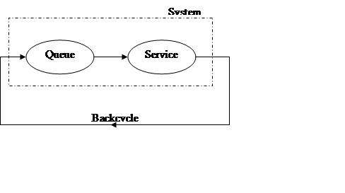
The usual tools then were regression, Petri nets, discrete-event simulation and genetic algorithms. Regression struggles with interactions and anything non-linear. Simulation needs the process to be well understood first. A neural network needs neither. It learns the mapping from examples. The price is that it needs a lot of good examples.
The data
The data had been collected earlier, by observation, for other research. Each pour had its own spreadsheet. For every truck it records:
- the batch, arrival, start and finish times;
- the load and the running total in cubic metres;
- the slump (a measure of how wet the concrete is);
- the inter-arrival, waiting, positioning and pumping times;
- the pump rate and the time the pump stood idle.
Each sheet also notes the date, the weather in a word, the mix, the part of the works being poured and the number of trucks on the job. The pours came from four wastewater treatment plant sites: Fraserburgh, Nigg, Hatton and Peterhead. They ran from 2 to 49 loads and from 1 to 14 hours.
I collected the usable pours into one summary sheet with Excel macros, dropped records with missing or corrupt data, and scaled every value to between 0 and 1. The pours were split 80:20 at random into training and testing sets. With so little data there was no separate validation set.
I built three input sets. All used the average inter-arrival, waiting, positioning and pumping times, average truck volume and slump. Then:
- Set A added the number of trucks, total volume and the month.
- Set B used the number of loads instead of trucks, and no month.
- Set C was set B plus the month.
Month was a crude stand-in for weather. I had collected Met Office station data but it never made it into the models.
The output was either the pour’s productivity or its total duration. Duration divided into total volume gives productivity, so predicting duration saves the network a step.
The method
All the networks were built with Matlab’s Neural Network Toolbox. I wrote programs that trained a network for every combination of size and transfer function, for each input set and each output, and recorded how well it did on the test pours. Results went into colour grids, one square per network.
There were six investigations:
- Radial basis networks, varying the one setting that matters (the spread) across nine orders of magnitude.
- Two-layer networks, first layer from 20 neurons down to 1, with every arrangement of linear, log-sigmoid and tan-sigmoid functions.
- Three-layer networks, both hidden layers from 20 down to 4.
- and 5. The best two- and three-layer networks again, now trained with regularisation or early stopping to stop them over-fitting.
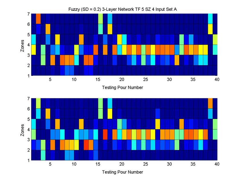
- “Fuzzy” networks that output a probability for each of seven productivity bands, rather than one number.
The fuzzy idea came from Portas and AbouRizk (1997). The same site conditions can give different productivities, so a range is more honest than a point. Where they spread the training targets with fixed values, I spread each observed pour as a normal curve, so the targets carried where in a band it fell.
What it found
Small networks beat big ones. On the training data, the larger the network the better the fit. On the test pours the order reversed. The large networks had learned the noise in 190 or so pours. This is over-fitting, and with this little data it dominated.
A linear network was hard to beat for productivity. Every all-linear network found the same answer, and it was a good one. Non-linear networks could do better, but less reliably.
Duration needed non-linearity. Linear networks predicted duration poorly. Three-layer non-linear networks predicted it very well across most sizes.
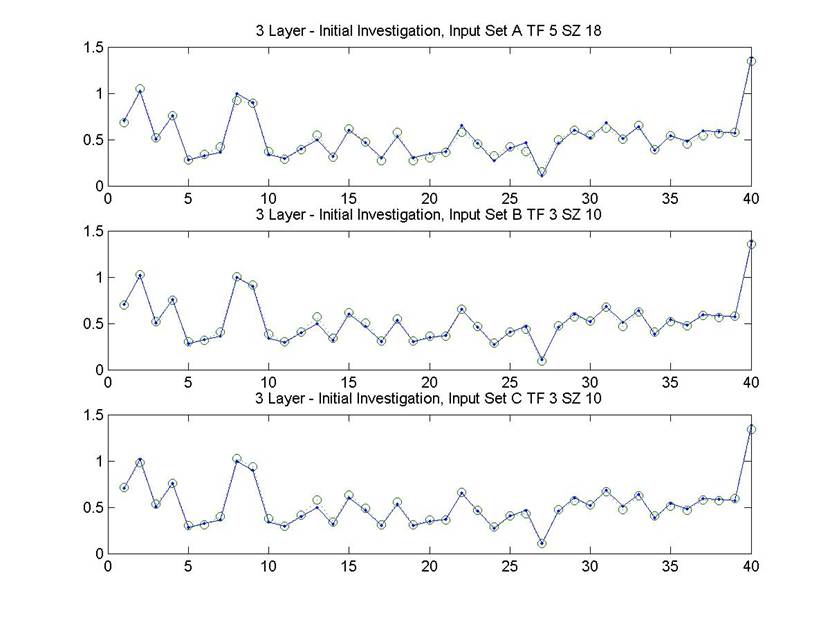
Regularisation and early stopping didn’t beat size reduction, but made success more likely. With them, even oversized networks usually generalised well, so far fewer had to be tried.
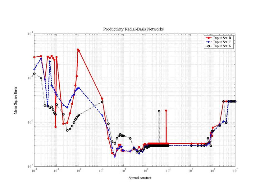
Radial basis networks were simpler to tune and a little worse. The best spread was about 40 to 100. Input sets B and C did best.
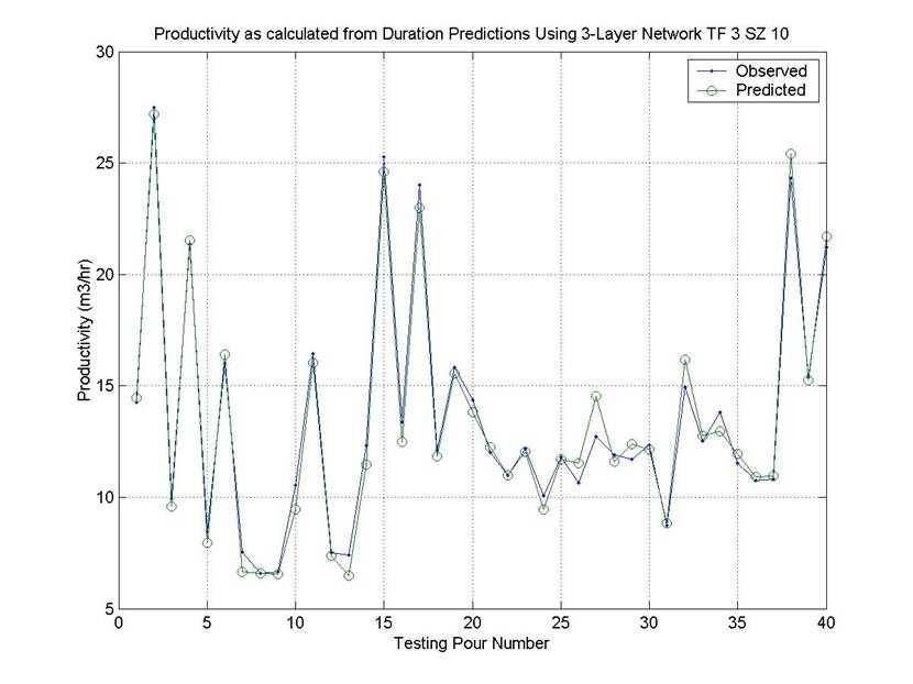
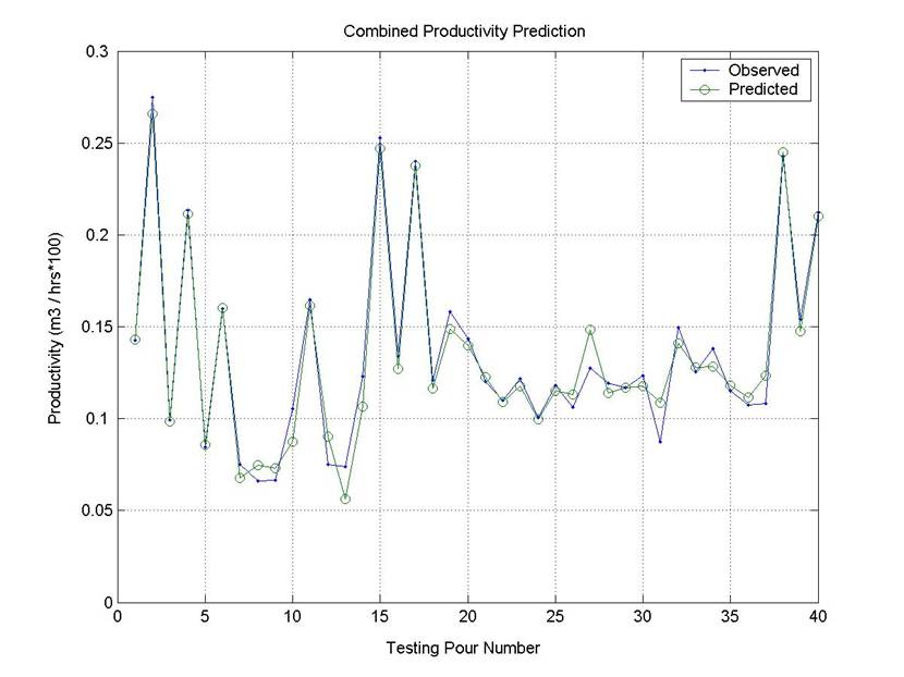
The best route to productivity went through duration. A three-layer network (16, 4 and 1 neurons) predicted each pour’s duration. Dividing the total volume by that gave productivity. It fitted the test pours better than any network that predicted productivity directly, and better than averaging the three best of those.
The banded output worked. The best three-layer fuzzy network put most of the probability in the right band, or the next one, for nearly every test pour.
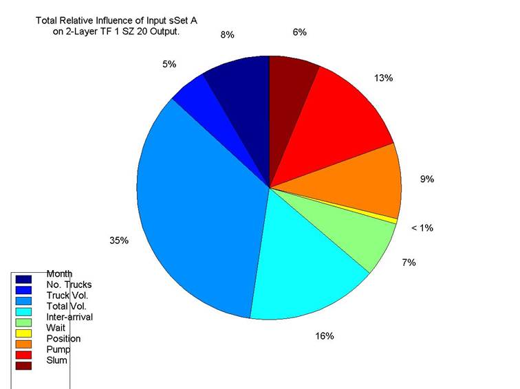
You can look inside a small network. I took the simplest good network — linear, two neurons then one — and traced how much each input moved its output. Total volume, truck volume and pumping time mattered most. That makes physical sense. The pump is the bottleneck, and the time lost per truck is roughly fixed, so bigger loads mean higher productivity. Waiting time and the number of trucks barely registered, but that is because they varied so little in real pours, not because they don’t matter.
What it showed, and what it didn’t
It showed that a neural network can learn the productivity of a stochastic construction process from site records. It also showed how much the answer depends on the data. All 239 pours came from one kind of project, in one region, over one year. Nothing here says how the networks would do on a new site, with new methods, or with estimated rather than measured inputs. The thesis said so, and argued that the real prize would be continuous data — telemetry on pumps and trucks — and weather.
The ideas I most wanted to try next were recurrent networks, which could follow each truck round its cycle, and networks built to mirror the physical process, with separate parts for separate sub-cycles.
How accurate
Error is measured on the forty test pours, as root mean square error, against an average productivity of 13 m³/hr:
| Network | Error | As a share of average output |
|---|---|---|
| Best networks predicting productivity directly | about 1.0 m³/hr | 8% |
| Three of those, averaged | about 0.9 m³/hr | 7% |
| Productivity worked out from predicted duration | about 0.6 m³/hr | 5% |
Most predictions sit within a cubic metre an hour of what happened. The one clear miss is a two-load pour lasting just over an hour.