One Formula, Many Worlds

A walk down to the determinant and back up to the broken Jacobian conjecture

A human–AI field expedition · August 2026

This is not an academic paper, and it does not pretend to prove anything new. It is the record of a pattern of thought: what happens when you take a famous, freshly broken conjecture, refuse to be satisfied with the headline, and climb all the way down to the most primitive object underneath it — then walk back up, rung by rung, watching one small formula reappear in richer and richer worlds. Along the way we will meet a formula that never changes, letters that keep upgrading what they mean, low-dimensional pictures that turn out to be honest shadows of something bigger, and one very specific place where ninety years of intuition fell over in 2026.

Part I · The primitive

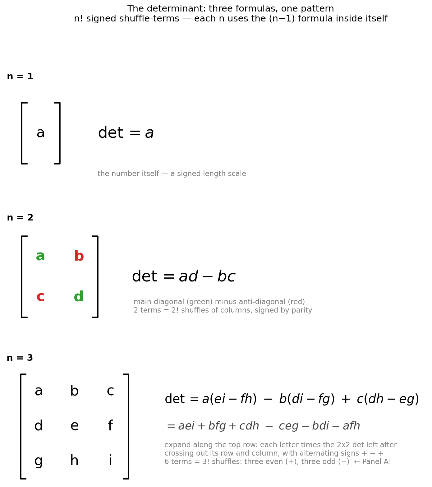
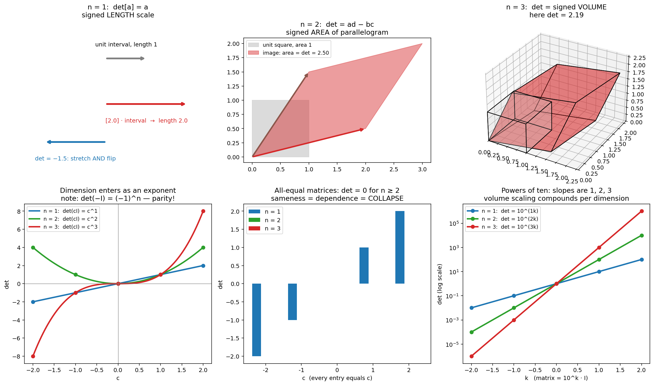
Strip everything away and a determinant is a single idea: a signed volume. A 1×1 matrix is just a number a, and its determinant is that number — the factor by which it stretches a length, with a minus sign if it flips direction. A 2×2 matrix has determinant ad − bc, which is exactly the signed area of the parallelogram its two columns span. A 3×3 matrix gives the signed volume of a parallelepiped. The sign carries orientation: positive means the transformation preserves handedness, negative means it works in mirror image.

Before the first picture, a word about tickets. Every theory quietly legislates what it accepts before it says anything at all, and the determinant is no exception: printed on its entry ticket, so faintly that generations read past it, is the clause let the entries commute. On the rungs we start from, the clause is invisible — numbers, formal variables and functions all commute automatically, so the legislation costs nothing and nobody thinks to mention it. But it is real: what the formula delivers is truth for these types of number, a quality defined at the door and holding across every dimension of the climb. Much later the expedition will meet the exact place where the clause starts to bind — the fork of Part III — and will find that the conjecture at the top of this story wears the same silhouette — the hidden hypothesis of Part V.

Playing with the simplest possible matrices already exposes three laws. First, sameness is collapse: a matrix whose entries are all equal — all 2s, all −1s, anything — has determinant zero the moment n reaches 2, because its rows are dependent and the volume flattens. Collapse cares about independence, never about size. Second, dimension enters as an exponent: scaling all of space by c scales the determinant by c to the power n — lengths by c, areas by c², volumes by c³ — so on a log plot the powers-of-ten families are straight lines of slope exactly 1, 2, 3. Third, and most delicious, parity: the matrix −I, which flips every axis, has determinant (−1)^n — a sign whose additive origin is taken up in Part V. Flipping everything is a rotation in even dimensions and a true mirror reflection in odd ones. The same recipe produces a different kind of transformation depending on the parity of the dimension. That is the smallest, cleanest instance of the theme that runs through this whole story: identical rules behave differently one dimension up.

Part II · The shuffle anatomy

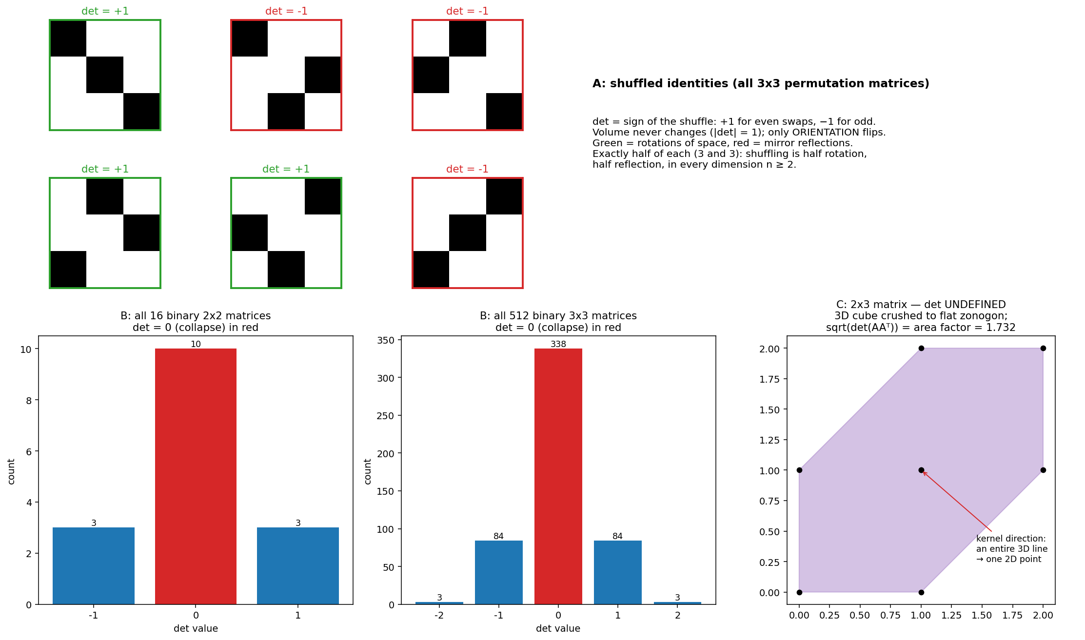
Where does the formula ad − bc actually come from? Shuffles. The determinant of an n×n matrix is a sum over all n! ways of picking one entry from each row so that no two share a column — non-attacking rooks — with each product signed by the parity of the shuffle that produced it: plus for an even number of swaps, minus for odd. The purest witnesses are the permutation matrices, identities with their 1s shuffled: every one of them has determinant exactly +1 or −1, volume untouched, only orientation at stake, and they split perfectly in half — shuffling axes is half rotations and half reflections, in every dimension.

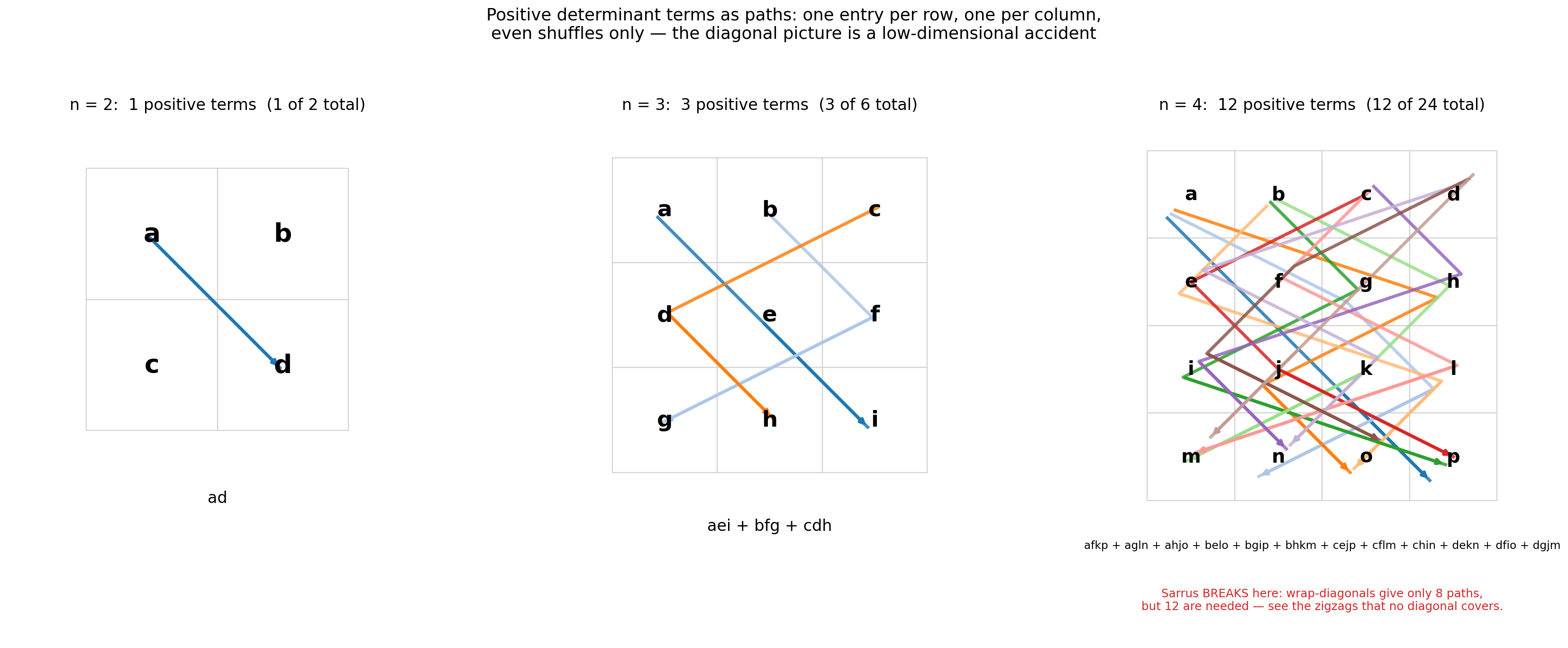
The signed shuffles can be drawn. Take the positive terms only and trace each product through the grid of letters: at n = 2 there is a single diagonal; at n = 3 the three positive terms are the main diagonal and two skewed outward arrows — the classical Rule of Sarrus, rediscovered by simply asking what the lines look like. And then n = 4 springs a famous trap: there are twelve positive terms but wrap-around diagonals can only supply eight paths, so the picture is forced into zigzags no diagonal covers. The diagonal rule was never the real object. It was a low-dimensional accident — a true shadow of the general rule (one entry per row and column, signed by parity) that the rule outgrows the moment there is room to zigzag.

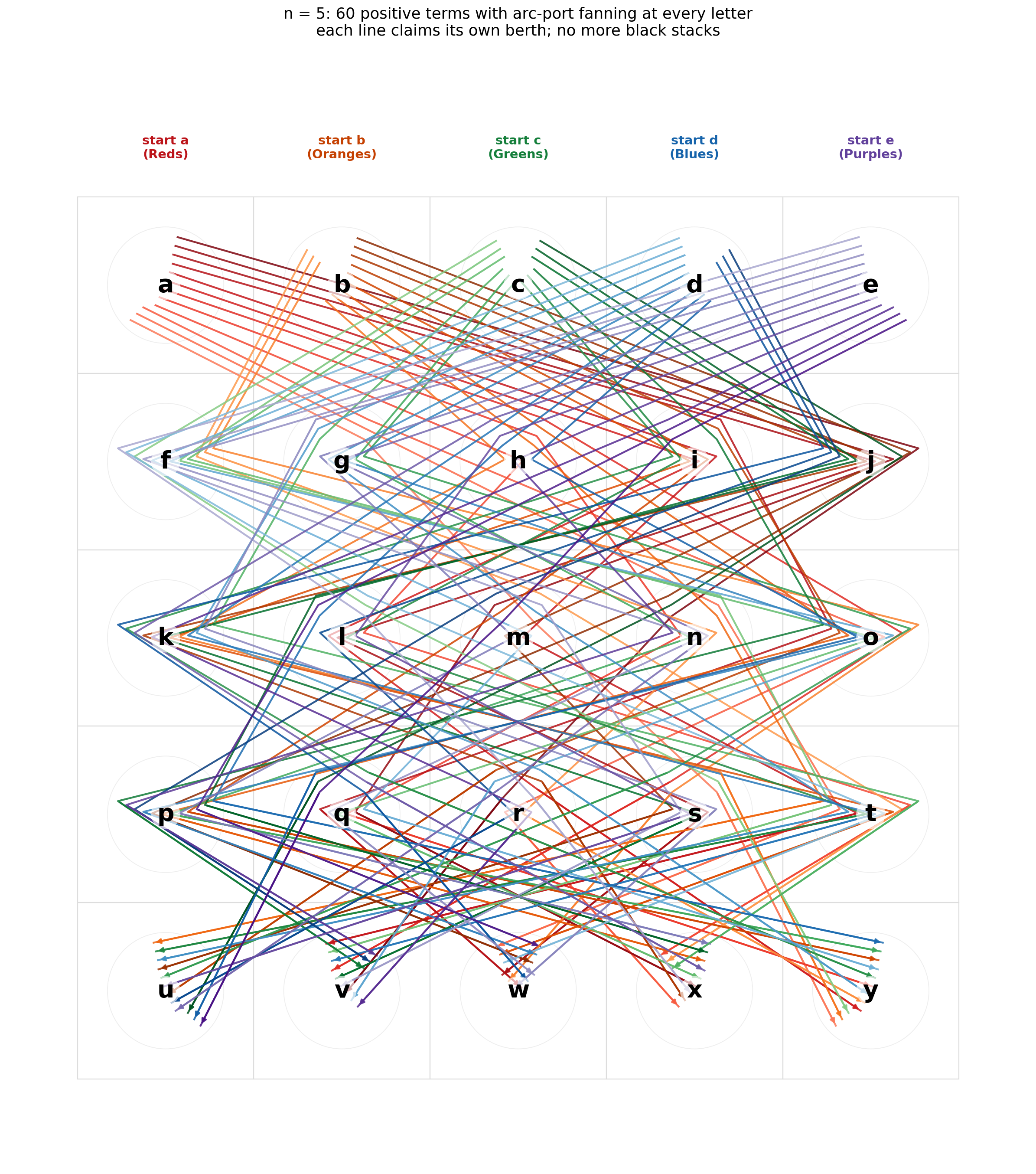
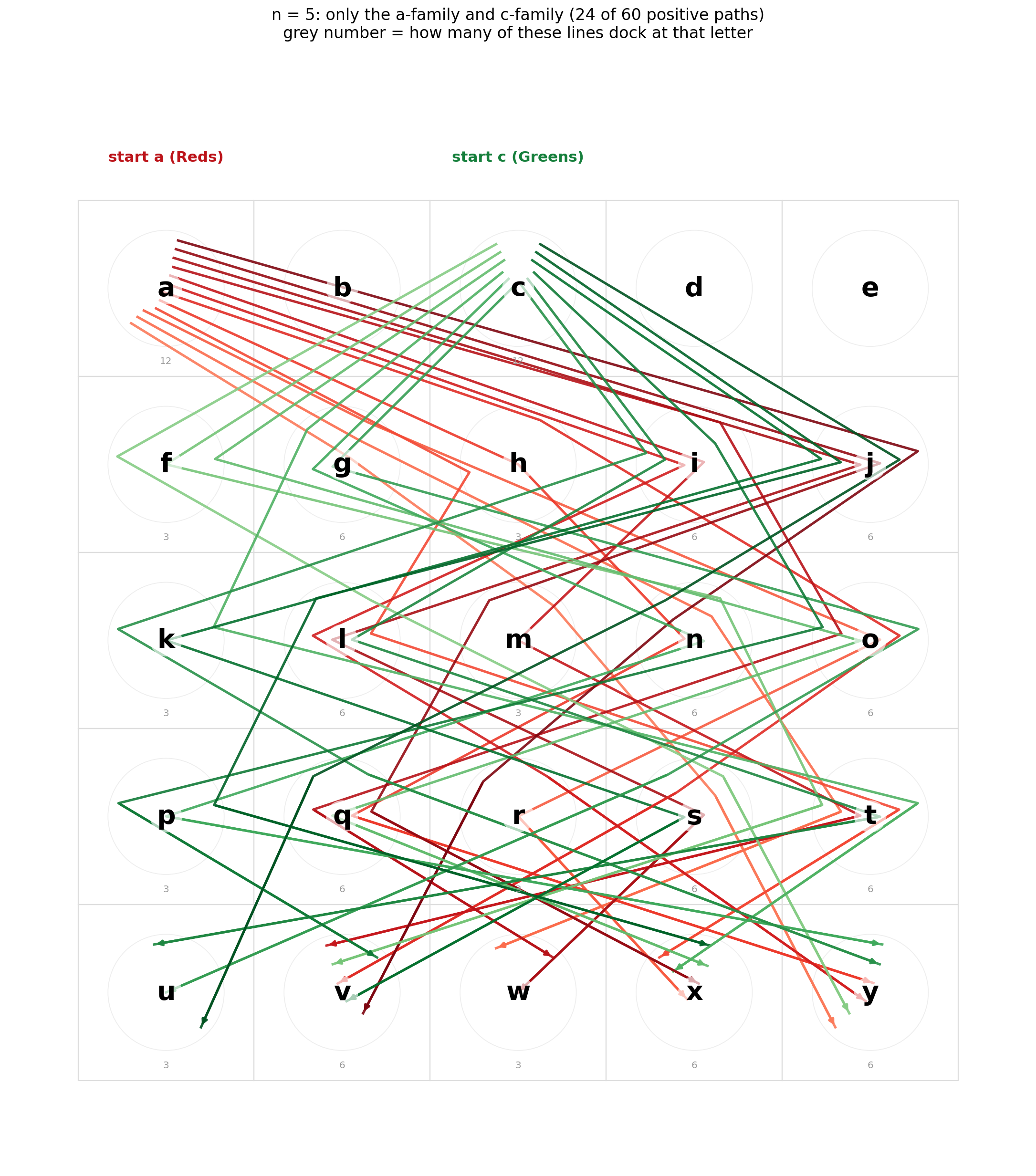
At n = 5 the positive half of the determinant is sixty paths, and drawing them all at once required inventing a rendering discipline: around every letter sits an invisible circle, and each line docks at its own berth along an arc perpendicular to its direction of travel, so parallel strands fan out instead of fusing into black. The fix accidentally proved a structural fact and made it countable by eye: every one of the twenty-five letters is visited by exactly twelve positive paths. The determinant is perfectly democratic — no entry of a matrix is privileged.

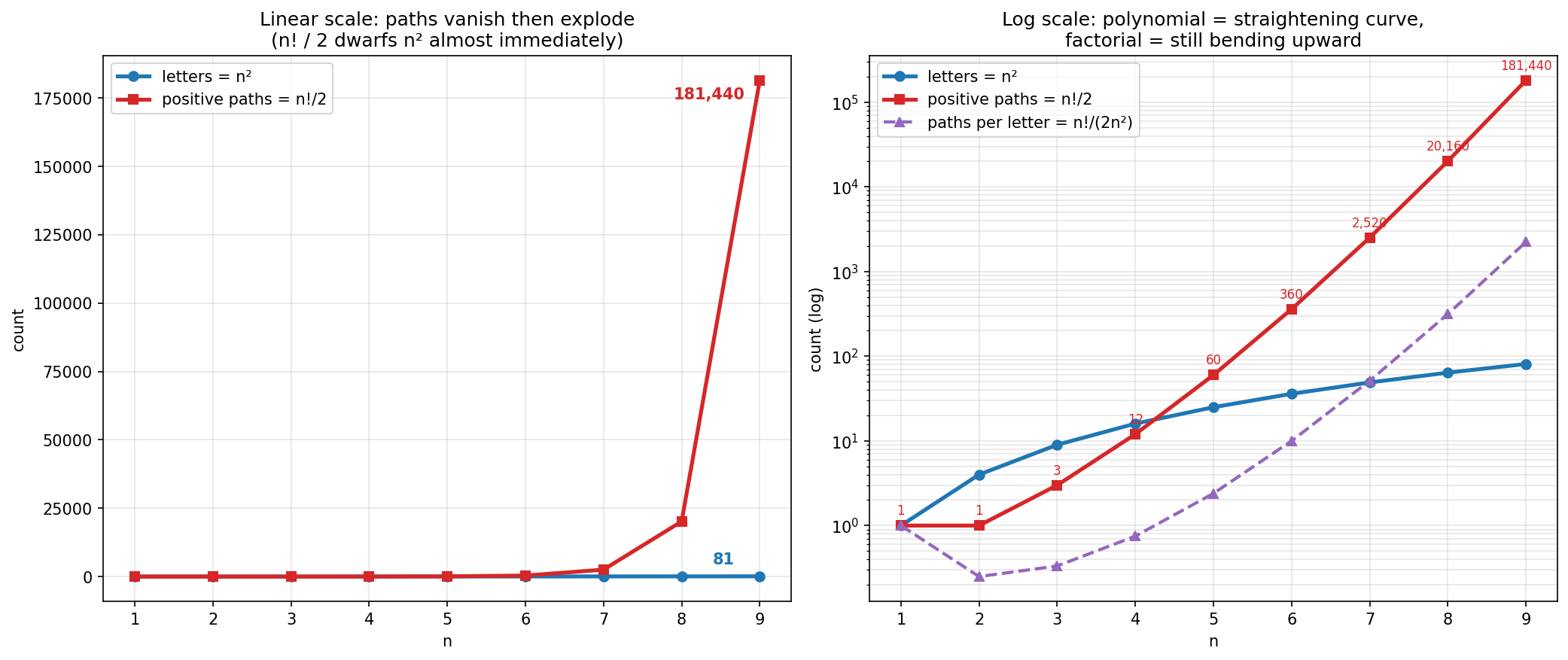
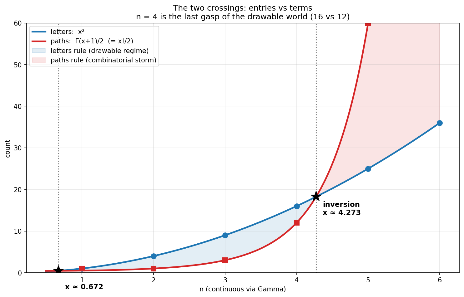
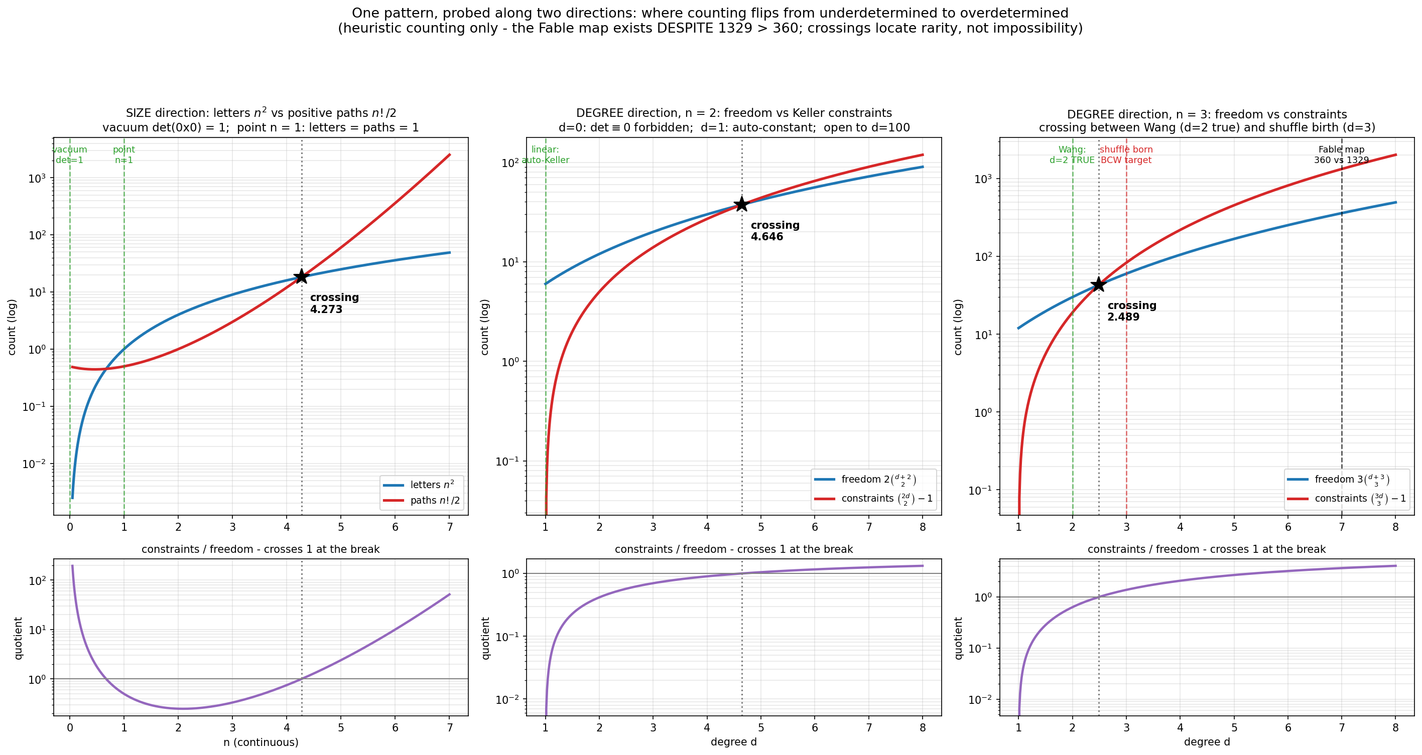
How do the two populations grow? Letters grow like n², a gentle polynomial. Positive paths grow like n!/2, a factorial. On a log plot the polynomial straightens out while the factorial keeps bending upward — factorial growth beats every polynomial ever. Extending the factorial smoothly between integers with the Gamma function, the two curves cross at x ≈ 0.672 and again at x ≈ 4.273. Between those crossings lies the drawable world, where entries outnumber terms and pictures like Sarrus’s are possible; n = 4 is its last integer citizen, and only barely, sixteen letters against twelve paths. After the inversion at 4.273 the combinatorial storm rules: by n = 9 there are 181,440 positive paths threading 81 letters, over two thousand paths per letter, and visual mathematics is dead.

Part III · The enrichment move

Here is the single most important structural observation of the whole journey, and it deserves plain words. The determinant formula never changes again. What changes, rung by rung, is only what kind of thing the letters are. First the letters are numbers. Then the same numbers are read as a transformation. Then — the move that creates calculus-flavoured mathematics — the letters become functions of position: each entry is a partial derivative ∂Fi/∂xj, different at every point of space, and the determinant stops being a number and becomes a field, a landscape of local volume-scaling draped over the domain. This is exactly what Carl Gustav Jacob Jacobi did in his 1841 paper on functional determinants, and his theorem was a dependence test: the field vanishes identically precisely when the functions are dependent. The right name for this repeating move is not recursion — the layer is not fed into itself — but enrichment: one primitive, re-instantiated over richer objects. It is arguably the master pattern of mathematics, and it does not stop here: above functions the same formula lives on as Fredholm determinants of infinite-dimensional operators and as the functional determinants physicists compute daily in quantum field theory.

One quieter rung deserves to be made explicit, because the ladder skips past it if you blink. Between number and function sits the variable: a pure formal symbol, an x that lives in a polynomial ring and obeys nothing but the laws of addition and multiplication. A determinant of variables is an identity — true wherever those symbols may later be sent, which is exactly why the formula cards of Figure 1 could be written once and for all. A function is the next rung up: the same symbol deployed over a domain, with a value at every point and a landscape you can draw. The two are easy to conflate and worth keeping apart, and they shelter under the same commutative-ring umbrella — a property so obvious it never seemed like an assumption, and which is about to become load-bearing.

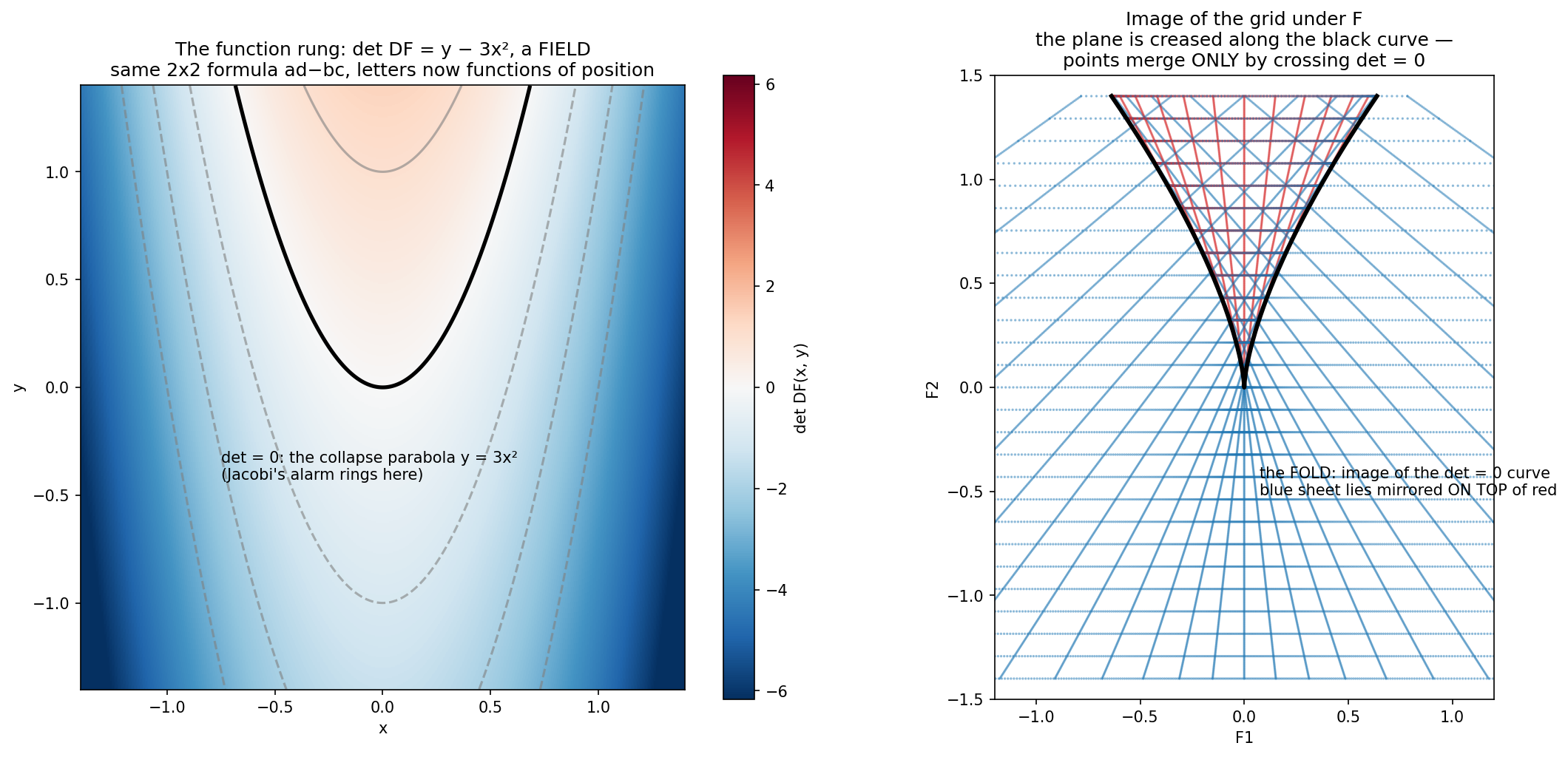
On the function rung the landscape has territories. Where the field is positive the map preserves orientation; where it is negative the map runs in mirror image; and the black curves where it is zero are the collapse locus — Jacobi’s alarm. The canonical example is the Whitney cusp map, whose determinant field is y − 3x², positive above a parabola, negative below. The map creases the plane like paper exactly along that parabola: the mirror sheet folds over and lands on top of the preserving sheet, and every point in the doubled region has two preimages. In this world, merging and collapse are the same event — points can only merge by crossing the alarm curve. Hold that sentence; it is about to matter.

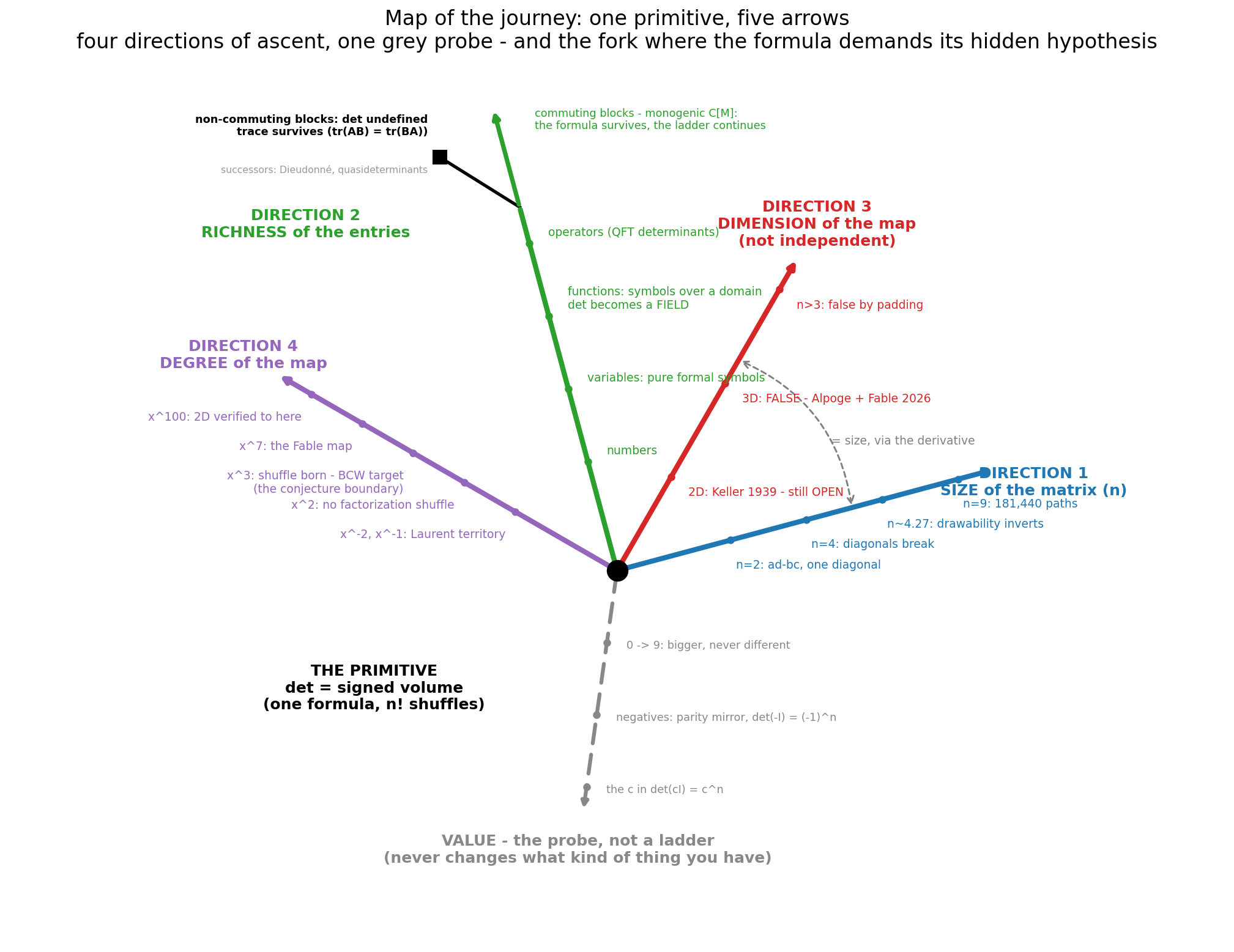
And the richness ladder has a fork. Keep enriching and the entries eventually become matrices themselves: a matrix of matrices, a block matrix. Along one branch nothing breaks at all: blocks drawn from a monogenic subalgebra C[M] — polynomials in one fixed matrix — commute among themselves, and the formula climbs on undamaged. The other branch is where the fall happens: generic blocks refuse to commute, and “the” determinant stops being well-defined — the familiar 2×2 recipe det(AD − BC) computes the true determinant of the underlying 4×4 only when the blocks commute, and over generic blocks it disagrees both with the truth and with its own mirror det(AD − CB). The determinant’s additive twin, the trace, walks straight past this fork: tr(A+B) = tr(A) + tr(B) always, and tr(AB) = tr(BA) holds even for non-commuting blocks. There are two true tellings of this event. In discovery order — the order this expedition lived — you climb, you fall, and you learn why the hypothesis exists. In legislation order, the textbooks’ order, the determinant is simply defined over commutative rings — the entry ticket of Part I, printed in advance — and within the stated domain nothing ever breaks: the theory is spotless, and the condition looks arbitrary precisely because the fall that explains it has been legislated away. Nor is the far side void: weaker successors live in non-commutative territory — the Dieudonné determinant over division rings, taking its values in an abelianised quotient, and the Gelfand–Retakh quasideterminants beyond that. The compass of Figure 0 draws the fork, and it is a different kind of boundary from every other threshold in this story: not a picture outgrown, but a hypothesis demanding to be seen.

Part IV · The flat landscape, and the break

The information ladder

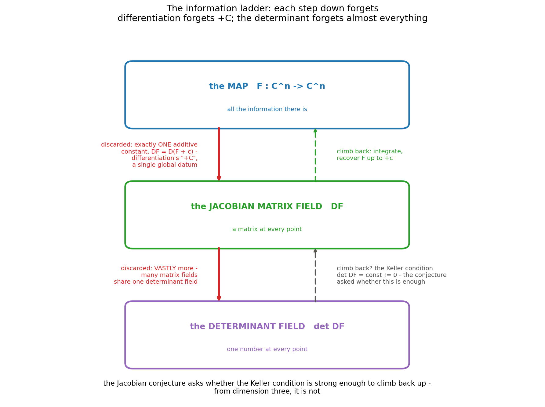
Before Keller’s question can even be asked, notice what it is made of: a chain of forgettings. Start from the map F itself — all the information there is. Differentiate, and you hold the Jacobian matrix field DF; what has been discarded is exactly one additive constant, since DF = D(F + c) — differentiation’s famous +C, a single global datum, recoverable by integration up to that shift. Take the determinant, and the second step discards vastly more: a whole matrix of partial derivatives collapses to one number per point, and countless different matrix fields share the same determinant field. The Jacobian conjecture lives at the bottom of this ladder and asks whether one scalar clause — the Keller condition, det DF equal to a nonzero constant — is strong enough to climb all the way back up to global invertibility. The counterexample answered: from dimension three, it is not.

Now the question almost asks itself, and in 1939 Ott-Heinrich Keller asked it. (The conjecture is named for Jacobi’s determinant, but Jacobi died in 1851, eighty-eight years before the question existed — with one gorgeous irony: his personal motto was man muss immer umkehren, one must always invert, and the conjecture bearing his determinant’s name is precisely the question of when inversion is guaranteed.) Suppose we forbid the alarm from ever ringing: take a polynomial map whose determinant field is one flat nonzero constant across the whole landscape. No zero curve, no crease line, no local collapse anywhere — the map is locally invertible at every single point. Must it then be globally invertible? In one dimension the answer is trivially yes; local and global coincide, there is no room between them. In two dimensions the answer is unknown to this day, verified for polynomials up to degree one hundred, resistant to ninety years of attempted proofs. And the general folklore, encouraged by results like the Bass–Connell–Wright reduction of the whole problem to degree-three maps, was that it ought to be true in every dimension.

In 2026 it broke. A counterexample in three dimensions — credited to the mathematician Levent Alpöge working with the AI model Claude Fable 5, announced in a social media post short enough to verify by hand — exhibits an explicit degree-seven polynomial map of C³ whose Jacobian determinant is exactly −2 everywhere, and which nevertheless sends three distinct points to the same image. We verified it ourselves, symbolically, in a few lines of computer algebra: the determinant is the constant −2, and F(0, 0, −1/4), F(1, −3/2, 13/2) and F(−1, 3/2, 13/2) all equal (−1/4, 0, 0). Remarkably, all three colliding points are real, so the collision can literally be seen: on the plane those three points span, the distance to the shared target has three separate wells.

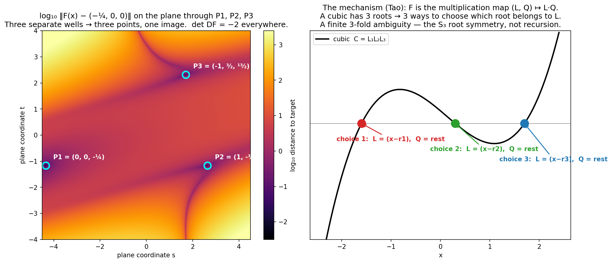
Why does it look like a miracle, and why is it not one? A degree-seven map of three variables has a Jacobian determinant that could a priori be a polynomial of degree eighteen — 1,329 coefficients that must all vanish, against only 360 coefficients of freedom in the map. Brute force should never find such a thing; that arithmetic is the shuffle storm of Part II wearing its adult clothing, and Figure 15 draws it along both the size and the degree axes. The published dissection, worked through on Terence Tao’s blog, reveals the trick: the map is secretly the multiplication of polynomials. Take a linear form L and a quadratic form Q in two variables; their product is a cubic. A generic cubic factors into three linear forms, and there are exactly three ways to decide which factor is L and which two belong to Q. The map is honestly three-to-one for the oldest reason in algebra: a cubic has three roots and they can be shuffled. The miracle was finding a slice of this multiplication map that is polynomially equivalent to plain C³. The kernel of the counterexample is not an infinite regress; it is the finite symmetric-group shuffle of three roots — the very same parity-and-shuffle object whose portrait fills Figures 3 through 6.

This diagnosis explains the dimension boundary. In the plane, the analogous product would be linear times linear equals quadratic — and a quadratic splits into two linear factors in only one way once scalings are normalised. Degree two has no shuffle. Degree three is the first place the ambiguity exists, and dimension three is where it first finds room to live on an honest copy of affine space. So the two-dimensional conjecture survives, and what died is only the belief that the gap between local and global invertibility is empty in high dimensions. Counterexamples travel upward by the dullest mechanism imaginable — pad with untouched dummy variables — so every dimension above three falls with the third.

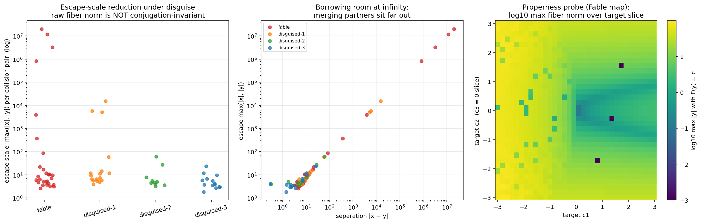
One more signature deserves its picture. When we built a numerical instrument to hunt collision pairs — pick a random point, solve for a different point with the same image — the partners it found were not nearby. They sat enormously far out, at coordinates of order ten to the seventh. That is non-properness in action: the map merges points by borrowing room at infinity, routing the identification through the far reaches that a bounded picture never shows. And it dovetails with the classical rescue theorems, because a proper map with nonvanishing Jacobian is a covering map of simply connected space and hence a bijection: properness is exactly the hypothesis that seals the escape route. In our computational sweeps, every map that collided had escaping fibers, and every properly-behaved map we could build had none. The instrument cannot prove theorems — its silence is evidence, never proof, and nobody yet knows how to generate Keller maps beyond the tame, invertible-by-construction families and disguises of the one known counterexample — but it points steadily at the same dividing line.

The degree axis

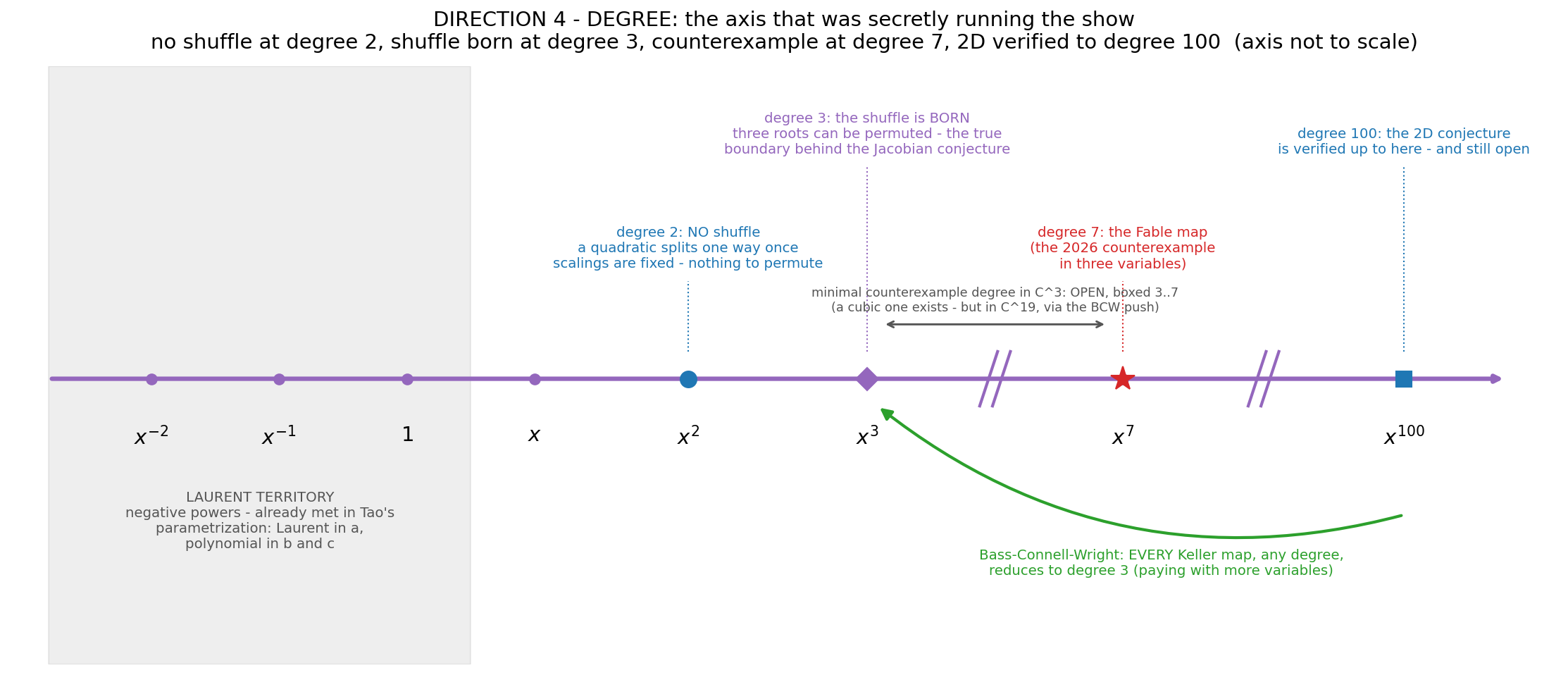
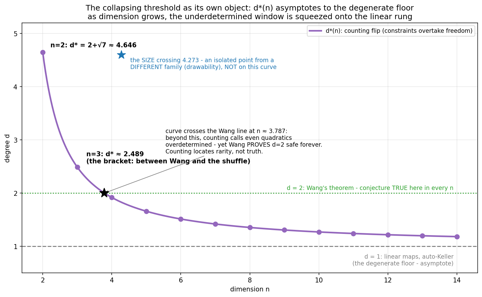
There is a fourth direction that has been running the show from behind the curtain, and it deserves its own arrow: degree. Every threshold of this Part sits somewhere on it. Degree two is barren: a quadratic form splits into linear factors in only one way once scalings are fixed, so there is no shuffle and nothing for a counterexample to be made of. Degree three is where the shuffle is born — three roots that can be permuted — and it is also, by the Bass–Connell–Wright reduction, where the entire problem lives: every Keller map of every degree can be pushed down to degree three at the price of more variables, so the whole axis collapses onto its first interesting point. Degree seven is where the 2026 counterexample actually sits — though seven is only where this construction landed: nobody has proven degrees three through six safe in three variables, so the minimal degree of a non-injective Keller map of C³ is itself open, boxed between three and seven (a cubic counterexample does exist, but in C¹⁹, via the Bass–Connell–Wright push). Degree one hundred is how far the two-dimensional conjecture has been verified by sheer computation, still without a proof. And the axis extends backwards past the constants into negative powers — Laurent territory — which already made a cameo in the dissection of the counterexample’s fibers: Laurent in a, polynomial in b and c. Counting hangs one more marker on the axis. A map of Cⁿ with components of degree at most d has n·C(d+n, n) coefficients of freedom, while the Keller condition demands C(nd, n) − 1 vanishings, and the point where the demands overtake the freedom falls at d = 2 + √7 ≈ 4.646 in the plane and at d ≈ 2.489 in space. The space value sits strictly inside the gap between Wang’s theorem — the conjecture is proven true for every map of degree at most two, in every dimension — and degree three, where the shuffle is born and the reduction lands: proven-true just below the crossing, mechanism-born just above it. Whether that bracketing is structure or numerology is a question this expedition can pose but not answer; the counting is a genericity heuristic in any case, and the counterexample itself sits at degree seven, deep on the overdetermined side of the flip. Value was a probe; degree is a genuine dimension of the problem, and the compass of Figure 0 gives it the fourth full arrow. One further observation, offered as observation and nothing more: the vertical axis of the quotient panels that accompany the crossings has its two distinguished values at the two vacuums — zero, the degenerate floor where the constraints vanish altogether (the additive nothing), and one, the balance line on which every crossing happens (the multiplicative nothing). In the low-dimensionality window the quotient lives between the two voids, and the smooth global trend only takes over once the curve escapes through 1.

Part V · What survives, and the shape of the pattern

So what, in the end, was reclaimed — and by whom? The honest scorecard reads like this. The determinant itself is untouched and eternal. Jacobi’s local theorem is untouched: nonvanishing determinant still means local invertibility, everywhere, in every dimension. The repaired global statements are genuine theorems that hold in all dimensions: an injective polynomial map is automatically bijective with polynomial inverse, and a proper locally invertible map is a bijection. The two-dimensional conjecture — the version Keller himself flagged as already hard in the plane — still stands, now sharper for knowing exactly which mechanism it must forbid: a candidate research programme, suggested by everything above, is that every failure of injectivity for Keller maps factors through a multiplication-type map with its root shuffle, a statement which in the plane would be vacuous and would therefore imply the surviving conjecture. Alongside it stand the other open problems this walk brushed against: the Hadamard maximal determinant problem, reachable with nothing but zeros and ones, and the search for a conjugation-invariant measure of non-properness that survives the disguise-compression of Figure 13.

The two vacuums

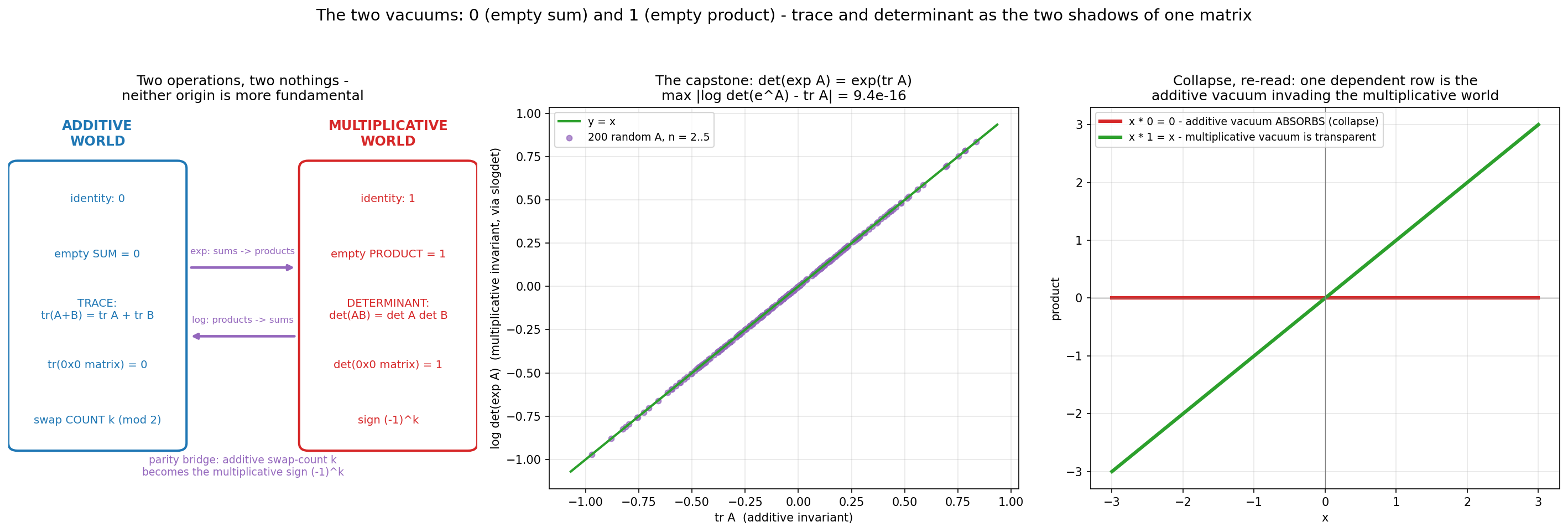
One last layer sits beneath everything above, and it surfaced from the most innocent question the expedition asked: do numbers start at zero or at one? The answer is that arithmetic has two origins because it has two fundamental operations, each with its own nothing. Zero is the additive identity, the value of the empty sum; one is the multiplicative identity, the value of the empty product. Neither is more fundamental — they are the ground floors of two different buildings. The determinant is a creature of the multiplicative building: det(AB) = det(A)·det(B), volume compounding by multiplication, which is exactly why the determinant of the empty 0×0 matrix is 1 and why det(I) = 1 — its vacuum had to be the multiplicative one. And it has an additive twin living in the same matrix: the trace, with tr(A+B) = tr(A) + tr(B) and an empty-matrix trace of 0. One matrix, two invariants, one per world — and the fork of Part III tells them apart: the multiplicative invariant breaks on the non-commuting branch, but the additive twin walks past the fork, because cyclicity, tr(AB) = tr(BA), never needed commutativity. Parity is the bridge between the buildings: counting swaps is additive bookkeeping, modulo two, but the determinant records the count multiplicatively as a sign, (−1)^k — every plus and minus on the rainbow paths of Part II is a multiplicative shadow of an additive swap-count. Exponentiation is the general machine that converts the additive world into the multiplicative one, and logarithms run it backwards. The capstone is a single line that holds the whole correspondence: det(exp(A)) = exp(tr(A)) — the multiplicative invariant of the exponential is the exponential of the additive invariant, a classical identity that follows from a formula which also carries Jacobi’s name. We ran it through the numerical instrument across two hundred random matrices and the largest discrepancy was of the order of machine precision — evidence in the instrument’s hands; the proof belongs to the textbooks. And with the two vacuums in hand, collapse itself reads differently. The additive nothing absorbs under multiplication — x·0 = 0, which is why a single dependent row kills an entire determinant, as the all-equal matrices of Figure 2 showed — while the multiplicative nothing is transparent: x·1 = x, felt by nothing. Collapse is the additive vacuum invading the multiplicative world. What happens when the visit runs the other way — the multiplicative nothing abroad in the additive world — is saved for the finale.

The hidden hypothesis

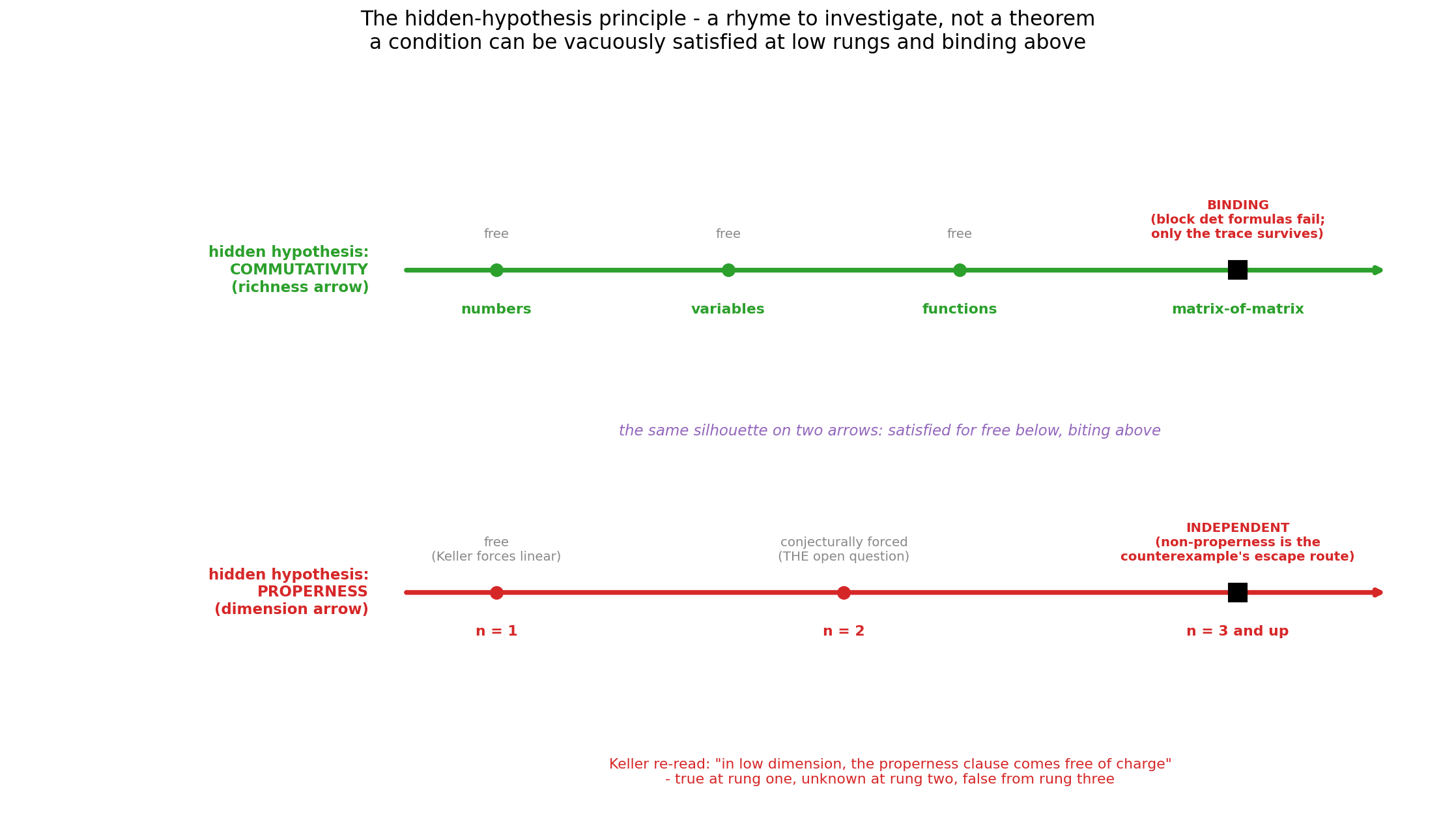
One more lens, and it may be the expedition’s most transferable find. The determinant’s theory silently carried commutativity as a standing hypothesis the whole way up the richness arrow: numbers, formal variables and functions all commute automatically, so the hypothesis was satisfied for free and nobody needed to state it — until the entries became matrices, where it binds, the block formulas fail, and only the trace continues. That is the general shape: a hypothesis can be vacuously satisfied at low rungs and binding above, so a theory can look unconditional for generations simply because nobody had climbed high enough to make its hidden condition bite. And the Jacobian conjecture wears exactly this silhouette on the dimension arrow — a rhyme to investigate, not a theorem. The candidate hidden hypothesis is properness. At n = 1 it comes free of charge: a Keller map of one variable is forced linear, hence proper, hence invertible, and the hypothesis holds invisibly. At n = 2 it is conjecturally forced: the open conjecture is exactly the claim that planar Keller maps cannot escape. From n = 3 it is demonstrably independent: the counterexample is a Keller map that is not proper, and non-properness is precisely its escape route, merging points by borrowing room at infinity. On this reading Keller’s conjecture was never “local implies global”; it reads as “in low dimension, the properness clause of the inversion theorems comes free of charge” — true at rung one, unknown at rung two, false from rung three. The repaired theorems of the scorecard above are the accepted-primitives framing of the same fact: legislate properness — or injectivity — onto the entry ticket, and invertibility holds spotlessly in every dimension. What that legislation quietly erases is exactly the open question, whether the plane grants properness free of charge. And this paper has now walked its own principle in three beats: the ticket legislated quietly in Part I, the fork discovered in Part III, the principle named here. The question the lens generates is concrete: find the weakest properness-flavoured condition that low dimensions grant automatically, and prove that the plane grants it.

The two nothings, complete

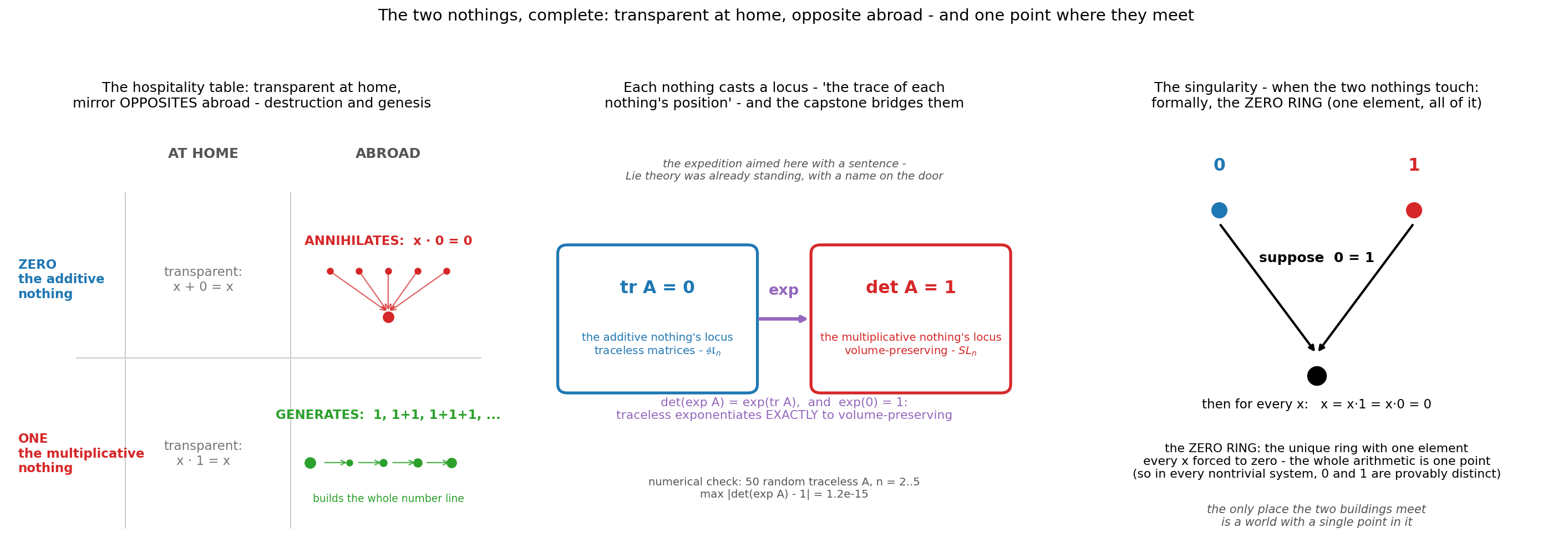
One piece of unfinished business remains, and it completes the two-vacuums layer — which is why we saved it for last. Each nothing, at home, is perfectly transparent: x + 0 = x, and x·1 = x — that is what being an identity means. The interesting behaviour is abroad. Zero, visiting the multiplicative world, annihilates: x·0 = 0, every element crushed to a single value — this is the collapse the whole paper has been telling, the dependent rows and all-equal matrices of Figure 2 seen one last time. But one, visiting the additive world, does the exact opposite. Adding 1 fixes nothing at all — x + 1 moves every element — and repeated addition of 1 builds the entire number line out of nothing: 1, then 1+1, then 1+1+1, and onward without end. The two cross-postings are mirror opposites, not symmetric copies: the additive nothing abroad is destruction; the multiplicative nothing abroad is genesis.

Inside the matrix world, each nothing also casts a shadow — the trace of each nothing’s position, in both senses of the word. The additive nothing’s locus is tr A = 0, the traceless matrices; the multiplicative nothing’s locus is det A = 1, the volume-preserving ones. And the capstone identity of the two-vacuums section, det(exp(A)) = exp(tr(A)), carries one locus exactly onto the other, because exp(0) = 1: traceless exponentiates precisely to volume-preserving. These two loci have standard names — sl_n and SL_n — and their correspondence under the exponential is a founding structure of Lie theory. The expedition aimed at this with one sentence and found the whole edifice already standing, with a name on the door.

And then the finale, which is a theorem-shaped fact and deserves to be stated like one. Ask what happens in a number system where the two nothings touch — where 0 = 1. Then for every x whatsoever, x = x·1 = x·0 = 0: every element is forced to zero, and the whole arithmetic contracts to a single point. This object exists and has a name — the zero ring, the unique ring with one element, the terminal degenerate case of all of algebra — and the derivation just given is the entire proof that in every nontrivial number system the two nothings are provably distinct. Call the coincidence a singularity if you like; algebra calls it the zero ring. It is the deepest degeneracy the value probe can reach — below the vacuum rungs of every other axis sits the one-point world, and the only place the two buildings ever meet is a world with a single point in it.

The ground floor

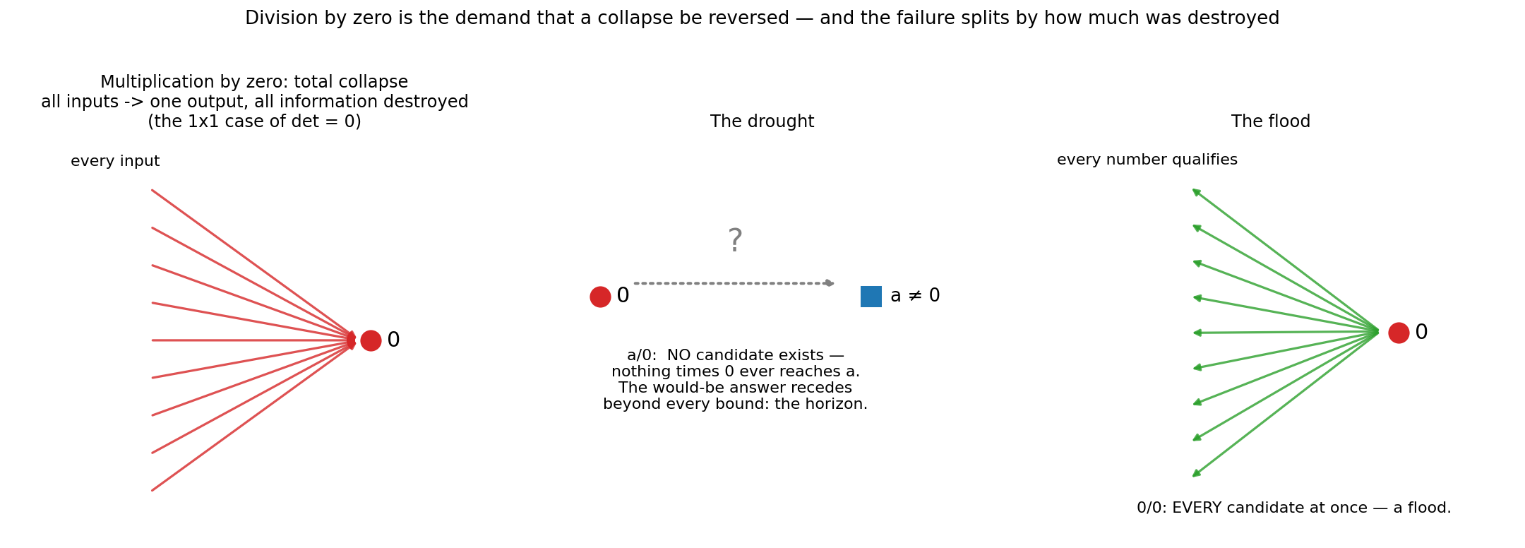
One more descent, prompted by the most schoolroom question of all, and it turns out to be the bottom rung of the entire ladder. “Undefined” for division by zero was never mathematics saying broken; it is mathematics saying there is no answer within this space — division is a partial operation whose entry ticket, like the commutativity ticket of Part I, simply does not admit a zero divisor. And the reason no answer exists inside is the oldest fact in this paper wearing its smallest costume: multiplication by zero is total collapse, every input crushed to one output, all information destroyed — the 1×1 case of det = 0 — and division by zero is the demand that the collapse be reversed. The failure even splits by how much was destroyed. For a/0 with a nonzero, no candidate exists at all: nothing times zero ever reaches a, and the would-be answer recedes beyond every bound toward the horizon of the previous section — which the Riemann sphere duly annexes as a point, selling a law of arithmetic to buy it. For 0/0, every number is a candidate at once: a flood in place of a drought. Two opposite failures, none-versus-all, both descendants of one annihilation. So the prohibition every child memorises without reasons is Jacobi’s dependence alarm sounding in its smallest possible instance — no collapse, and inversion is locally guaranteed; collapse, and inversion dies — and from that rule to the conjecture that fell in 2026 is one ladder with no missing rungs. The full descent into the counterexample’s own geometry — the valleys, the mirror in the fiber, the two branches, the hole with its drapery, and the two horizons — is the business of the field appendix, Down the Needle, which dives from this section’s floor.

And the humans? The counterexample is credited to a human mathematician working with an AI model, and the aftermath was gloriously human: verification by hand within hours, because the example is small; a geometric explanation reconstructed on a blog; arguments in the comments about which formulation was ever the fundamental one; and a mechanical push of the example through the classical reduction machinery within days. If there is something to reclaim, this expedition suggests it is not priority but understanding — the thing this document is made of. A search process found the needle; the meaning of the needle, the shuffle at its heart, the parity in its sign, the escape route through infinity, and the primitive at the bottom of it all were recovered by exactly the kind of walk anyone can take: downward to the simplest object, then up one enrichment at a time, drawing pictures until the pictures break, and paying attention to precisely where and why they break.

Because that is the repeating shape, seen now from both ends of the ladder — and the compass we drew at the start has its final form: five arrows. Value, greyed and dashed, the probe that never changes what kind of thing you have, only how much of it. Size of the matrix, where the pictures live and die. Richness of the entries — numbers, variables, functions, operators — climbing to the commutativity fork, where non-commuting matrix-of-matrix entries cost the formula its meaning while the trace survives. Degree, the axis that was secretly running the show: barren at two, fertile at three, broken at seven, verified to one hundred. And dimension of the map, which was never independent at all — it is size seen through the derivative, tethered to the first arrow by the chain rule. One formula, unchanged. Low-dimensional pictures — the diagonal, the fold — that are true shadows of the general rule until the rule outgrows them at a sharp, computable threshold: diagonals die at four, folds stop being the only merging mechanism at three, drawability inverts at 4.273. Parity deciding character: rotation or reflection by the evenness of n. Collapse always meaning dependence, never size. And at every rung, the gap between what is locally guaranteed and what is globally true — empty at the bottom, conjectural in the plane, and, as of 2026, provably inhabited from dimension three upward, by a shuffle that was sitting in the 2×2 formula all along — and beneath it all, two vacuums: the additive zero that absorbs, the multiplicative one that the determinant calls home — and, at the bottom of everything, the one-point world where the two nothings coincide and arithmetic itself closes its eyes.

Epilogue · Where the ladder goes

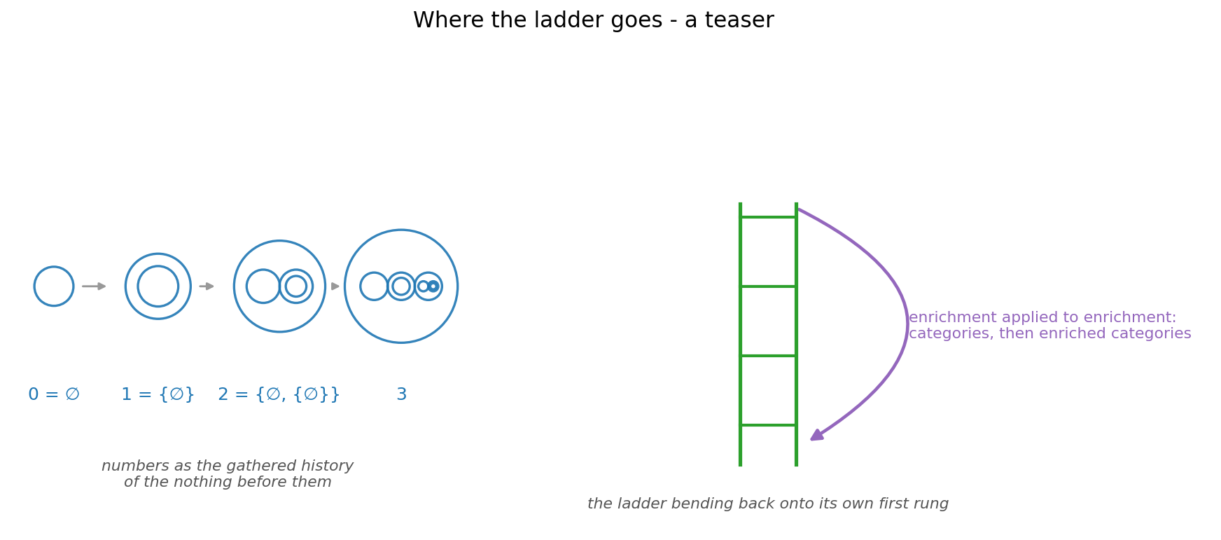
One door remains, and it opens outward. The expedition’s very first instinct — that this story would turn out to be self-eating recursion — was wrong about the Jacobian mechanism, which is a finite shuffle and no regress at all, and right about the method: the enrichment move applies to itself. Modern foundations build the numbers from generative nothing — 0 = ∅ and 1 = {∅}, the set containing nothing, each number the gathered history of everything before it. And taking the ladder itself as the object of study is already a living branch of mathematics, whose own vocabulary — enriched categories — keeps the metaphor honest. That walk is Paper II — and it starts, as this one did, at nothing.

Appendix · Provenance and computation

Every figure in this document was generated during the expedition by short Python scripts (numpy, sympy, scipy, matplotlib), collected in the companion module determinant_ladder.py, which reproduces all of them through a numeric menu. The counterexample map, its constant Jacobian, and the triple collision were verified symbolically with sympy. The explicit map and its geometric dissection follow the public write-up on Terence Tao’s blog (July 2026); the counterexample is credited to Levent Alpöge with Claude Fable 5 (Anthropic), and at the time of writing the full prompt history and workflow of its discovery had not been made public, with formal peer review pending. The numerical collision hunts and properness probes are evidence-gathering instruments, not proofs, and are labelled as such wherever they appear.

← All notes · More from Maths Rooms