Scheme options - realistic reservoirs, no reservoir, and several smaller ones
Generated by build_scheme_options.py. The three follow-ups to sizing.
Generated by build_scheme_options.py. The three follow-ups to sizing.
The sizing sweep found a reservoir optimum at 10 Mm3 - the volume at which spill reaches zero. That is not a usable answer, because much above 5 Mm3 is not a realistic cell on this ground. So the questions become: what can be done under a realistic cap, what happens with no reservoir at all, and what about several smaller schemes?
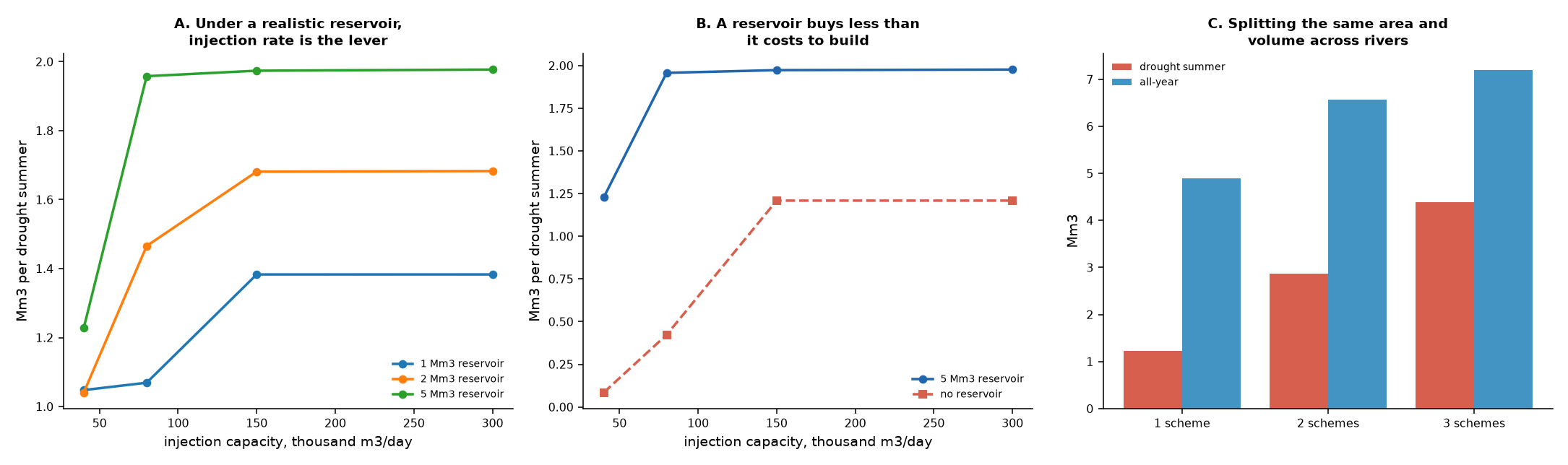
1. Under a realistic cap, injection rate is the lever
A reservoir exists to hold water while the wells accept it slowly. At 40,000 m3/day the wells take 4 Mm3 over a 100-day winter, so a flood arriving at 150,000 m3/day must be stored or lost. Enlarging the reservoir and raising the injection rate buy the same thing - they both close the gap between how fast water arrives and how fast it can be put underground.
| reservoir | injection m3/day | drought summer Mm3 | spilled Mm3 |
|---|---|---|---|
| 1 Mm3 | 40,000 | 1.05 | 39.3 |
| 1 Mm3 | 80,000 | 1.07 | 17.2 |
| 1 Mm3 | 150,000 | 1.38 | 11.6 |
| 1 Mm3 | 300,000 | 1.38 | 11.6 |
| 2 Mm3 | 40,000 | 1.04 | 28.0 |
| 2 Mm3 | 80,000 | 1.47 | 11.0 |
| 2 Mm3 | 150,000 | 1.68 | 8.1 |
| 2 Mm3 | 300,000 | 1.68 | 8.1 |
| 5 Mm3 | 40,000 | 1.23 | 9.5 |
| 5 Mm3 | 80,000 | 1.96 | 3.3 |
| 5 Mm3 | 150,000 | 1.97 | 2.8 |
| 5 Mm3 | 300,000 | 1.98 | 2.8 |
1.23 Mm3 per drought summer at the buildable baseline (5 Mm3, 40,000 m3/day) rises to 1.98 Mm3 at 300,000 m3/day on the same 5 Mm3 cell - a 1.6x gain from wells rather than earthworks.
That is the practical finding of this chapter. The project has swept reservoir volume repeatedly and never once varied the injection rate, which on this evidence is the cheaper axis and the more effective one. It also has the better failure mode: wells can be added incrementally, a reservoir cannot.
The edge case, for reference only
What would it take to catch all the winter water? 10 Mm3 spills 0.0 Mm3 and delivers 1.47, 20 Mm3 spills 0.0 Mm3 and delivers 1.09, 40 Mm3 spills 0.0 Mm3 and delivers 0.82.
Spill reaches zero around 10 Mm3, which is twice the practical ceiling. Full winter capture is not available on this ground with one cell, and the honest conclusion is that the scheme should be designed to take a share of the winter surplus rather than all of it.
1b. The intake pump, which dominates everything
This axis had never been swept, and it is the largest lever in the layer. It was found by accident - the portfolio comparison in section 3 originally left each sub-scheme with a full intake pump, so three schemes quietly had three times the intake. That alone produced an apparent 3.9x ‘portfolio advantage’. Giving a single scheme the same intake reproduces the gain and beats the portfolio.
| intake m3/day | drought summer Mm3 | spilled Mm3 |
|---|---|---|
| 150,000 | 1.23 | 9.5 |
| 300,000 | 3.67 | 86.4 |
| 450,000 | 4.66 | 126.3 |
| 600,000 | 5.18 | 139.4 |
Tripling the intake more than quadruples drought delivery, on the same basin, the same wells and the same mound. Nothing else in this project comes close - injection rate gave 63%, reservoir volume gave 65%, and the portfolio gives nothing at all.
The physics is the seasonality. 86% of the divertible resource arrives November-March and floods last days, not months, so the binding constraint is how fast you can take water while it is briefly there. A scheme that cannot lift it fast enough watches it go past, which is exactly what the rising spill column shows - the bigger pump captures far more even while spilling far more.
The caution is that this is the axis with the least modelling behind it: an intake at 450,000 m3/day is a substantial structure on the river, and nothing here checks whether the channel, the licence or the ecology would tolerate abstraction at that rate. It is the most promising and least investigated direction in the layer.
2. No reservoir at all
diversion: direct_inject: true pumps the river straight into the wells, and the reservoir disappears. This required a model change - recharge was previously drawn only OUT of the reservoir, so a zero-reservoir scheme had no injection path and delivered exactly zero, which was plumbing rather than physics.
| injection m3/day | with 5 Mm3 reservoir | direct, no reservoir | difference |
|---|---|---|---|
| 40,000 | 1.23 | 0.08 | -93% |
| 80,000 | 1.96 | 0.42 | -78% |
| 150,000 | 1.97 | 1.21 | -39% |
| 300,000 | 1.98 | 1.21 | -39% |
Direct injection reaches 1.21 Mm3 per drought summer at 300,000 m3/day, with no reservoir at all.
The reservoir earns its keep only where injection is slow - it buffers a flood the wells cannot swallow. Once the wells are fast enough to take the flood as it arrives, the cell is carrying very little, and on this evidence a scheme built around well capacity rather than surface storage deserves serious consideration. It also sidesteps the two things that make a reservoir expensive here: the land take, and the evaporation off a shallow cell on flat ground.
The obvious caution: direct injection has no settlement and no buffer, so raw river water goes to the wells at whatever turbidity the flood carries. Clogging is the standard failure mode of injection wells and nothing in this project models it. A real design would need at least a settlement stage, which is a small reservoir by another name.
3. Several smaller schemes
Total well-field area and total reservoir volume held constant and divided N ways, each sub-scheme on its own river. Two effects pull against each other:
- splitting helps capture - each sub-scheme has its own intake, and no single river carries more than 23% of the resource;
- splitting hurts retention - leakage goes as 1/r^2, so halving a mound’s area roughly doubles its fractional loss.
| schemes | radius each | reservoir each | injection each | half-life | drought summer Mm3 |
|---|---|---|---|---|---|
| 1 | 2.00 km | 5.00 Mm3 | 40,000 m3/d | 1,554 d | 1.23 |
| 2 | 1.41 km | 2.50 Mm3 | 20,000 m3/d | 777 d | 2.87 |
| 3 | 1.15 km | 1.67 Mm3 | 13,333 m3/d | 518 d | 4.38 |
It is the pumps, not the rivers
A pump is per-intake plant - you cannot share one between three rivers 30 km apart, so a real portfolio has one at every site. That means the per site rows below carry three times the intake capacity of the single scheme, and the comparison has to be made at equal total pumping before it means anything.
| configuration | total intake m3/day | drought summer Mm3 |
|---|---|---|
| 1 scheme | 150,000 | 1.23 |
| 1 scheme | 300,000 | 3.67 |
| 1 scheme | 450,000 | 4.66 |
| 1 scheme | 600,000 | 5.18 |
| 2 schemes, own pumps | 300,000 | 2.87 |
| 3 schemes, own pumps | 450,000 | 4.38 |
| 2 schemes, shared pump | 150,000 | 0.76 |
| 3 schemes, shared pump | 150,000 | 0.78 |
At equal total pumping the single scheme wins. 450,000 m3/day on one river delivers 4.57 Mm3; the same 450,000 split across three rivers delivers 4.32. The portfolio’s apparent advantage was three pumps against one, and the ~5% it gives back is the 1/r^2 leakage penalty on the smaller mounds.
That is a better answer than a portfolio, not a worse one. The gain you were chasing is real and roughly 4x - it is just bought with an intake pump on one river rather than with three schemes, three sites and three sets of consents.
The control, which changes what the result means
Splitting across three rivers is two changes at once: smaller mounds (worse) and more intakes (better). Running the same split all on the Tone isolates them:
| schemes | across rivers | all on one river |
|---|---|---|
| 1 | 1.23 | 1.23 |
| 2 | 2.87 | 1.07 |
| 3 | 4.38 | 0.95 |
The one-river column is the leakage penalty on its own. Whatever it does, it does without any gain in resource access. The difference between the two columns is what the extra rivers are worth.
The extra intakes more than pay for the faster leakage - which makes sense in a catchment where the resource is spread across nine rivers and no single one dominates. It also spreads the risk: three schemes on three rivers do not all fail in the same drought.
What this does not settle
- No costs. Wells, pipelines, land and earthworks all differ per option and none is priced. The direct-injection result in particular is a water result, and its case rests on well cost against reservoir cost.
- Clogging. The single biggest risk to a well-led scheme, and entirely unmodelled.
- One compartment’s properties. Every sub-scheme uses the Sherwood parameters. A real portfolio would use compartments with genuinely different behaviour - the Chalk holds water for decades but can barely accept any - and that mix is the next thing to test.
- Nesting. The three river systems are treated as independent. Isle and Parrett are not fully independent of each other downstream, so the portfolio total is slightly optimistic.