Sizing - what each scheme delivers when it is needed most
Generated by build_scheme_sizing.py. A capability curve, not a recommendation.
Generated by build_scheme_sizing.py. A capability curve, not a recommendation.
The demand layer settled a question that decides what this chapter measures. Licensed demand is 3.19 Mm3/yr; the water that could physically do good here is ~108 Mm3/yr on the arable alone. Demand is not the binding constraint, so % of demand met is the wrong statistic - it divides by an arbitrary denominator and saturates at 100%, hiding exactly the differences between sizings that the choice depends on.
So demand here is set deliberately high and never binds. Each configuration delivers as much as it physically can, and is scored on volume delivered in April-September of the drought years (WY2011, WY2015, WY2017, WY2022 - the water years under half the mean resource).
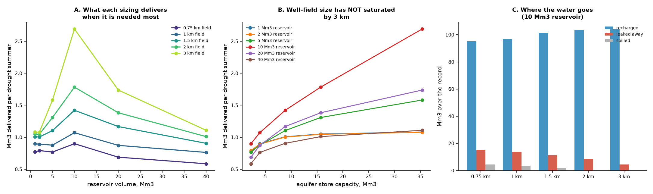
The curve
| well field | store Mm3 | half-life d | reservoir Mm3 | drought summer Mm3 | all-year Mm3/yr |
|---|---|---|---|---|---|
| 0.75 km | 2.2 | 219 | 1 | 0.77 | 2.08 |
| 0.75 km | 2.2 | 219 | 2 | 0.79 | 2.60 |
| 0.75 km | 2.2 | 219 | 5 | 0.77 | 3.69 |
| 0.75 km | 2.2 | 219 | 10 | 0.90 | 4.36 |
| 0.75 km | 2.2 | 219 | 20 | 0.69 | 4.11 |
| 0.75 km | 2.2 | 219 | 40 | 0.59 | 3.43 |
| 1 km | 3.9 | 389 | 1 | 0.90 | 2.66 |
| 1 km | 3.9 | 389 | 2 | 0.89 | 3.16 |
| 1 km | 3.9 | 389 | 5 | 0.88 | 4.03 |
| 1 km | 3.9 | 389 | 10 | 1.07 | 4.54 |
| 1 km | 3.9 | 389 | 20 | 0.87 | 4.30 |
| 1 km | 3.9 | 389 | 40 | 0.76 | 3.71 |
| 1.5 km | 8.8 | 874 | 1 | 1.01 | 3.58 |
| 1.5 km | 8.8 | 874 | 2 | 1.00 | 4.04 |
| 1.5 km | 8.8 | 874 | 5 | 1.10 | 4.68 |
| 1.5 km | 8.8 | 874 | 10 | 1.42 | 4.91 |
| 1.5 km | 8.8 | 874 | 20 | 1.17 | 4.70 |
| 1.5 km | 8.8 | 874 | 40 | 0.91 | 4.28 |
| 2 km | 15.7 | 1,554 | 1 | 1.05 | 3.76 |
| 2 km | 15.7 | 1,554 | 2 | 1.05 | 4.27 |
| 2 km | 15.7 | 1,554 | 5 | 1.31 | 4.98 |
| 2 km | 15.7 | 1,554 | 10 | 1.78 | 5.19 |
| 2 km | 15.7 | 1,554 | 20 | 1.38 | 4.92 |
| 2 km | 15.7 | 1,554 | 40 | 1.01 | 4.52 |
| 3 km | 35.3 | 3,497 | 1 | 1.08 | 3.87 |
| 3 km | 35.3 | 3,497 | 2 | 1.08 | 4.41 |
| 3 km | 35.3 | 3,497 | 5 | 1.58 | 5.18 |
| 3 km | 35.3 | 3,497 | 10 | 2.69 | 5.43 |
| 3 km | 35.3 | 3,497 | 20 | 1.74 | 5.13 |
| 3 km | 35.3 | 3,497 | 40 | 1.11 | 4.68 |
What the curve says
Every well-field radius has the same optimum reservoir: 10 Mm3. Above and below it, drought delivery falls. That consistency across five independent aquifer sizes is what makes it a result rather than a coincidence, and the mechanism is visible in the ledger:
| reservoir Mm3 | recharged | spilled | drought summer Mm3 |
|---|---|---|---|
| 1 | 73 | 39 | 1.08 |
| 2 | 83 | 28 | 1.08 |
| 5 | 99 | 10 | 1.58 |
| 10 | 104 | 0 | 2.69 |
| 20 | 98 | 0 | 1.74 |
| 40 | 89 | 0 | 1.11 |
Below 10 Mm3 the loss is spill. A 1 Mm3 cell spills 39 Mm3 over the record - it simply cannot hold a winter flood long enough to inject it. Above it the loss is evaporation. Recharge falls from 104 Mm3 to 89 Mm3, because water that sits on a larger surface leaves as vapour instead of going into the ground.
The optimum is the volume at which spill reaches zero. Buy less and you throw winter water over a weir; buy more and you buy evaporating surface. That is a satisfying result because it is a rate-matching argument, exactly as the scheme README predicted: the reservoir exists to hold water while the aquifer accepts it slowly, and the right size is the one that just covers the mismatch.
Well-field radius has not saturated
At the optimum reservoir, delivery rises 0.90 -> 2.69 Mm3 as the field grows 0.75 -> 3 km, and it is still climbing at the largest size tested. No optimum radius was found, so none should be read off this table.
The aquifer chapter warned why the sweep stops there anyway: past about 2 km the radial-flow idealisation is describing a well field larger than most of the compartments it would sit in, and the real limits - land, wells, and the body’s own edges - arrive before the arithmetic does. A3 is 16 km2; a 3 km field is 28 km2 and does not fit. Treat the 2 km row (1.78 Mm3) as the largest physically sited option on that compartment.
The oversizing penalty rests on an assumed depth
Reservoir area here is volume/5, i.e. a flat 5 m mean depth, which is what drives the evaporation penalty above the optimum. That is an assumption, and it is optimistic. The project has measured stage-volume-area curves for eight real sites and S1 has a mean depth of 2.96 m at 5 Mm3 - shallower, so more surface per m3 and a sharper penalty. Re-running this sweep against the measured curves would move the optimum down, not up.
Where the water goes
Panel C is the honest accounting. Across the record, most of what is diverted does not reach a field - it leaks back to the river from the store, or spills from a full reservoir. That is not a fault in the scheme; an unconfined store leaks by definition and 80% of that leakage is credited back as river baseflow, which is part of the environmental objective rather than a loss to the catchment. But it does mean the headline diverted volume is a poor guide to delivered water, and only the delivered column should be used for value.
What this chapter does not do
- It does not recommend a scheme. It is a capability curve. Choosing a point on it needs the value of water to a crop at a moment, which the demand layer cannot yet supply - the avoid crop failure tier needs crop coefficients and a yield-response function.
- It does not cost anything. Well-field area, reservoir fill and pipeline length are all proxies here, not costs. Cost is the axis that turns this curve into a decision.
- It sweeps two variables. Pump rates, injection limit, hands-off flow and intake location are all held at run 07’s values, and at least the injection limit deserves its own axis given panel C.
- The store is one compartment. A3 was chosen in availability as the best-placed body; a portfolio across compartments is a different and probably better scheme.
- Acceptance rate is bounded, not modelled. Nothing in 14 years of record contains an injection, so every injection-limited result here inherits that.