Storing winter river water underground on the Somerset Levels
The Somerset Levels have too much water in winter and not enough in summer. The rivers that cross them carry large flows from October to March and fall away by July, while the…
The first full paper, and the oldest document here. It predates the scheme layer entirely. The current statement of this work is Banking winter water for a dry summer.
What the scheme could deliver, what it depends on, and what we would have to measure to know
1. The problem, and the opportunity
The Somerset Levels have too much water in winter and not enough in summer. The rivers that cross them carry large flows from October to March and fall away by July, while the demand for irrigation water peaks exactly when the rivers are lowest. Surface reservoirs are one answer. Putting the winter water underground — into rock that already holds water — is another, and it avoids evaporating the store away in the summer it was built for.
This paper assesses that second option using only openly published data. It is a water-accountancy study: it tracks where every cubic metre goes, day by day, for sixteen and a half years of real river flow.
The regional context matters, because it tells you whether this is a good place to try. A screen of southern England — from Somerset to Kent, the south coast to the Thames — was run over 374 river-flow gauges, asking where three things coincide: winter river water that a licence would allow you to take, an aquifer nearby that could hold it, and a regulatory setting that does not forbid it.
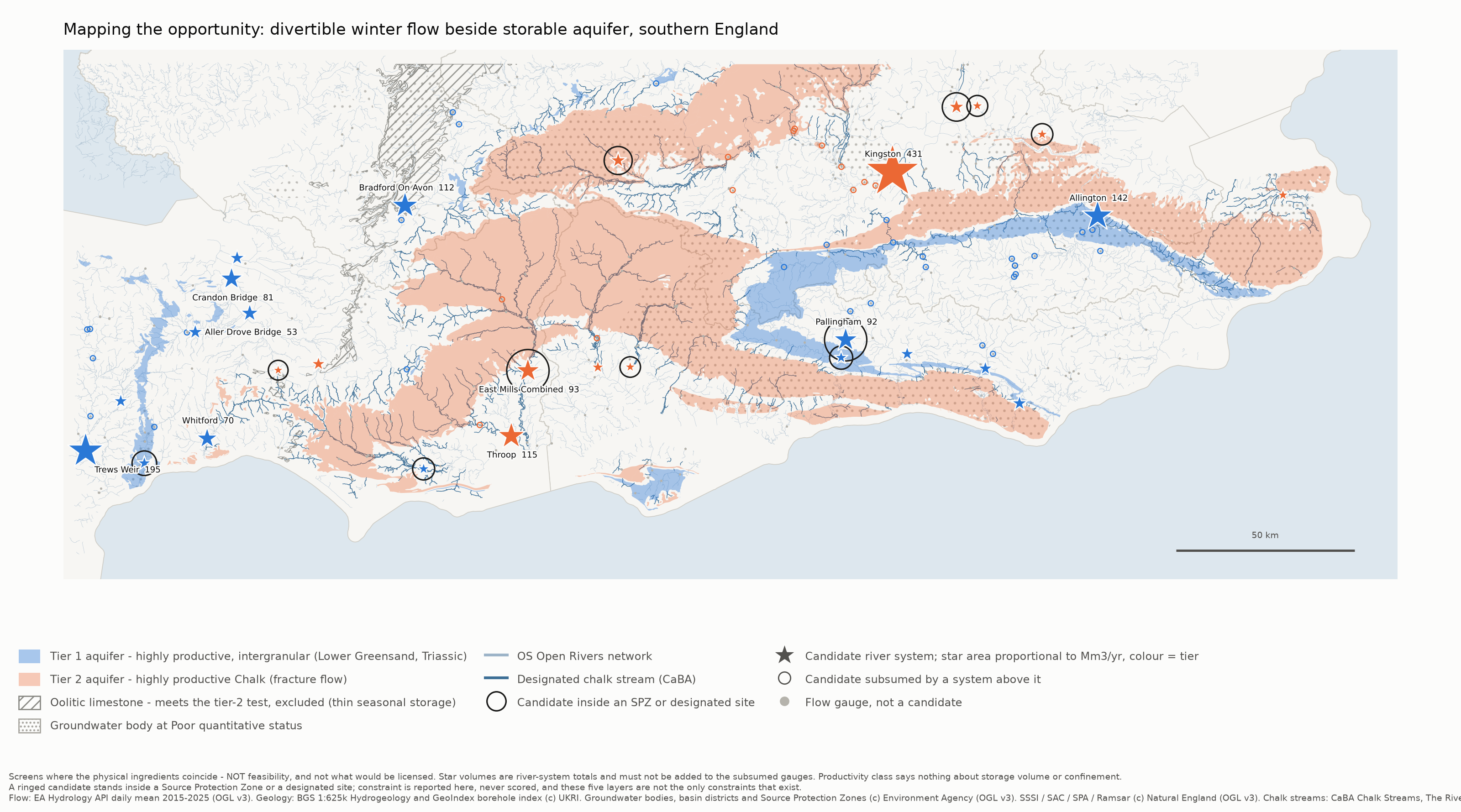
Figure 1. Where divertible winter flow sits beside storable aquifer across southern England. Star area is proportional to the water a licence-shaped rule would permit; colour is the aquifer type nearby; a black ring marks a candidate standing inside a protected site or a groundwater Source Protection Zone. Does not show: how much water any aquifer could hold, whether it would retain it, or whether a scheme would be permitted. Blank areas are places with no gauge, not places with no opportunity.
Two results from that screen frame this paper.
Somerset’s opportunities are among the least constrained in southern England. Of the twenty-eight independent river systems that cleared the screen, only six sit outside every protected site and away from every groundwater protection zone — and three of those six are in Somerset. In a region where the largest opportunities are inside European wildlife designations or inner groundwater protection zones, that is a real advantage.
The competition is mostly chalk, and chalk is politically exposed. Eight of the region’s candidates sit within fifty metres of a designated chalk stream. Somerset’s candidates sit on sandstone instead, which is both a different kind of aquifer and a much quieter place to work.
So the question this paper asks is not “is Somerset the best place in England” — it is “Somerset is a plausible place; what would a scheme there actually deliver, and what does that depend on?”
2. The data
Everything below comes from published sources. Nothing is commercial and nothing is confidential.
| What | Source | How far it can be trusted |
|---|---|---|
| River flow, daily, 2010–2026 | Environment Agency Hydrology API, eight gauges | Measured. Good. Fifteen days of a 6,025-day record were gap-filled. |
| Ground surface, 1 m | Environment Agency LiDAR | Measured, but covers only 58% of the study area |
| Ground surface, 50 m | Copernicus, reprocessed | Complete coverage, coarser detail |
| Which rock is where | British Geological Survey, 1:625,000 | Reliable for what the rock is; far too coarse for siting |
| How the rock behaves | — | Not available. See below. |
| Boreholes drilled | BGS GeoIndex | Locations and depths only — no rock descriptions, no yields |
| Protected sites | Natural England | Authoritative |
| Groundwater protection zones | Environment Agency | Authoritative |
| Rivers and canals | Ordnance Survey Open Rivers | Authoritative for where channels are |
The gap that matters most
No published open dataset says how well the target aquifer holds water. The BGS aquifer-properties layer was checked directly: it records where the Geological Survey holds such data, and contains no values — no storage coefficient, no permeability, nothing numeric. Four separate routes to the numbers were tried and all four returned the same answer.
This is not a detail. It is the single largest uncertainty in the whole assessment, and Section 6 shows that it moves the answer more than every design choice put together.
What already exists
Before assuming everything must be built, we looked for capacity that is already there. Within the study area, Ordnance Survey records 103 km of canal — including 17.6 km of the Bridgwater and Taunton Canal — and 929 separate stretches of standing water. The Huntspill River, an artificial channel already operated for water management, runs for 8.5 km; the King’s Sedgemoor Drain for 16.0 km.
None of it can be given a volume from open data. Published mapping gives the extent of water bodies, never their depth, and no open product publishes lake outlines for this area at all. So this is an inventory of what exists, not a store that can be counted on. It is included because it bears on a question the paper returns to in Section 10: whether finding somewhere to put the water is really the hard part.
3. The model
What it does
A daily ledger. For each of 6,025 days it works through a fixed sequence: read the river flow; decide how much may be taken under the licence rule; add it to the surface storage cell; take off evaporation; move water from the cell through treatment and into the aquifer; let the aquifer leak; pump water back out to meet irrigation demand; release water to the river when the river is low; and draw the cell down in autumn to leave room for winter.
The licence rule is the shape a real abstraction licence takes: do not start pumping until the river is running high, and never draw it below a floor. Both thresholds are set by how often the river exceeds them — the trigger at the flow exceeded 12.5% of the time, the floor at 19% — so the rule keeps the same stringency whatever the river is doing.
What it cannot do
It is not a hydraulic model. It has no channel routing, no groundwater flow field, no water quality, no sediment and no clogging of the injection wells over time. The aquifer is represented as a bucket that leaks in proportion to how full it is — which captures the behaviour that matters here (water put in drains away at some rate) without pretending to know where the water goes underground.
It also cannot tell you whether anything would be permitted, whether the land could be bought, or what any of it would cost.
How it is verified
Every run is checked for mass balance: water in must equal water out plus the change in storage, to within a cubic metre. Across the 141 runs in this paper the worst discrepancy was 0.000002 m³ — two millionths of a cubic metre over sixteen years. A synthetic self-test with a constant river runs on every change to the code.
One correction is worth recording because it changed results. The eight gauges used here are eight, not nine: a ninth gauge was found to measure a stream already counted inside another, so its water was being added twice. Removing it changed the water actually delivered by nothing at all, and capture by 0.5% — which is itself a finding, and Section 4 explains why.
4. What has already been established
Four things are known well enough to build on, and they are ordered by how much they move the answer.
1. How the aquifer behaves dominates everything. The same scheme, on identical inputs, meets 95% of irrigation demand if the store leaks slowly and 63% if it leaks at the rate actually observed in local boreholes. No design decision in this paper comes close to that.
2. Capture is set by the scheme, not by the river. Doubling the estimated river flow reduces the water captured, because holding the licence at the same stringency raises the trigger and the scheme can still only pump so much per day. Pump utilisation sits at 7–8% either way. Finding more water in the catchment does not help a scheme that is already limited by its own plant. This is why removing the double-counted gauge changed nothing.
3. Getting water out matters more than getting it in. Increasing the capacity to recover water raised reliability from 66% to 93%. A comparable increase on the injection side moved it by less than a point. They are not symmetrical.
4. Flood control is not on the table. Across the twenty largest flood events in the record, the scheme reduces the peak by a median of 1.4%, and at best 2.2%. The arithmetic caps it: a full day of pumping is about 3 m³/s against flood peaks of 100–300 m³/s. This is a water-resource scheme with an incidental flood benefit, and should never be presented as flood management.
The terrain result that changed the scheme’s shape
Storage on flat ground is a bunded box, not a dammed valley, so its cost is the ring of embankment around it. Searching the surveyed ground for sites gave an unambiguous answer:
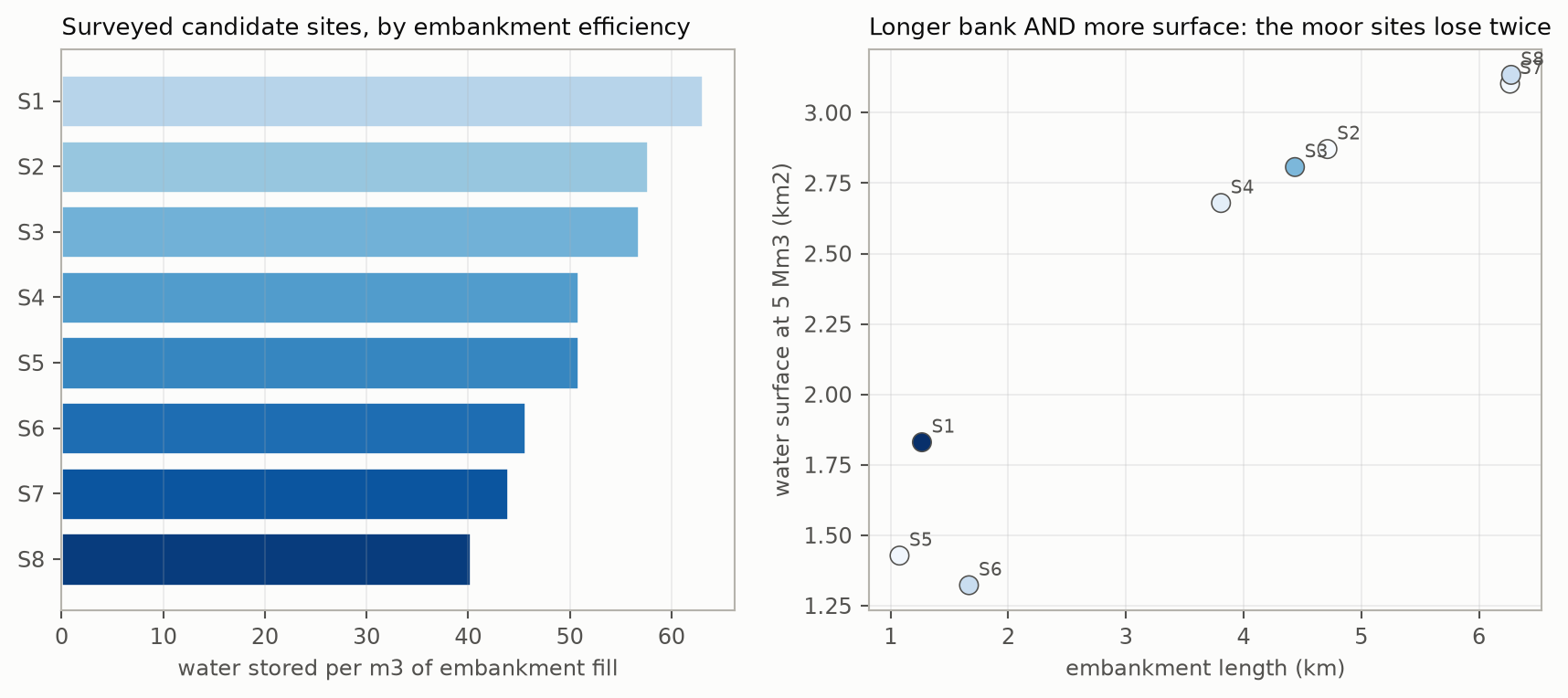
Figure 2. Left: the eight surveyed candidate sites ranked by how much water each stores per cubic metre of embankment fill. Right: embankment length against water surface area — sites on the open moor need a longer bank and expose more water to evaporation. Does not show: ground conditions, peat depth, seepage, land ownership, or whether any site could be consented.
A cell on the open moor needs five times the embankment of one in a natural hollow at the moor’s edge — 6.3 km of bank against 1.27 km for the same 5 million cubic metres. Flat ground gives the bund no help. The best site sits on mineral ground above the moor, which also avoids the peat, seepage and buoyancy problems of the low ground.
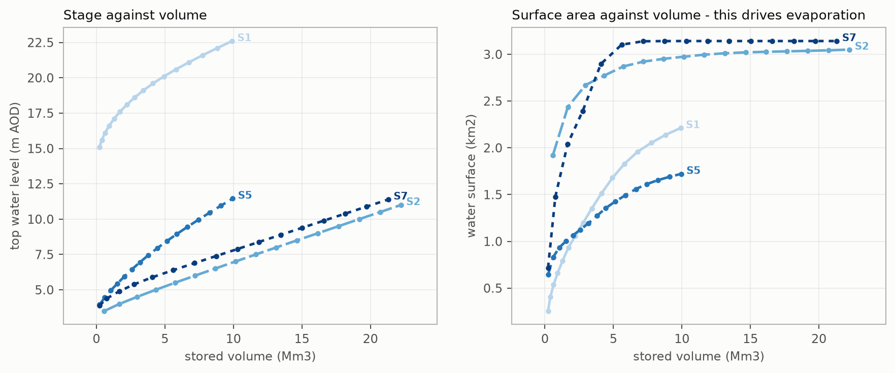
Figure 3. How much water each site holds at each water level, and the surface area that goes with it. Does not show: foundation conditions, freeboard for wave action, or land availability.
Figure 3 also shows a hard limit that is easy to miss: the best surveyed site cannot hold more than 9.9 million cubic metres, however much money is spent. Beyond that the ground runs out. Reservoir capacity is not a free design choice.
Looking wider than the survey
The surveyed area covers 58% of the study region and was drawn on the assumption — since disproved — that storage would sit on the moors. The search was therefore repeated on the complete but coarser 50 m terrain model.
The coarse search was validated first. Run over the surveyed area, it recovered all four leading fine-resolution sites, locating them within 355 m, with volumes and areas within 10% and efficiencies within 14% (the coarse grid is slightly optimistic). The coarse terrain can be trusted to find sites, if not to design them.
Run over the whole region, it found something the surveyed search could not have: the best site anywhere is one the LiDAR does not cover.
| Site | Efficiency | Distance to river | Lift | Surveyed? |
|---|---|---|---|---|
| C1 (E353525 N124725) | 88.1 | 1.5 km | 3.1 m | no |
| C2 (E380775 N118725) | 73.5 | 3.8 km | 11.8 m | no |
| C3 = best surveyed site | 67.6 | 3.6 km | 13.4 m | yes |
C1 stores 30% more water per cubic metre of bank than the best surveyed site, and sits closer to the river with a quarter of the lift. It lies inside the surveyed area’s boundary but in a gap in the survey.
Three further checks were run on C1, and it passed all three. It has zero overlap with every statutory designation, tested at those layers’ own resolution rather than the terrain model’s. It has less watercourse crossing it (2.0 km) than the baseline site used throughout this paper (3.8 km). And the coarse-model bias was measured against the four sites that exist at both resolutions — the 50 m model reads efficiency about 4% high, spread from −7% to +14% — so C1’s corrected efficiency is 85, and even at the pessimistic bound of that spread it is 77 against the best surveyed site’s 63.
C1 remains indicative until surveyed, and only a survey can find a road embankment, a quarry or a grid artefact in the hollow. But the two 1 m tiles needed (ST52nw, ST52sw) cannot currently be fetched: the Environment Agency’s download service has been decommissioned and every path now returns “Invalid URL”. They remain available by hand from the survey portal, and that is perhaps ten minutes of work for the largest single improvement available to this scheme.
One caveat that emerged from those checks applies to the whole candidate table: no site was screened for minor watercourses, and two surveyed candidates have the Parrett or the Tone crossing their footprints.
5. A baseline scheme
To see what each unknown does, we need something to vary. This is the starting point: a deliberately ordinary configuration, one store, every number justified.
| Element | Value | Why this number |
|---|---|---|
| Reservoir site | best surveyed | highest embankment efficiency with no conveyance conflict |
| Reservoir capacity | 5 Mm³ | mid-range of what the terrain allows (site limit 9.9 Mm³) |
| Water surface | 1.69 km² at capacity | from the surveyed terrain, not assumed |
| Diversion trigger | 30.6 m³/s | the flow exceeded 12.5% of the time |
| Hands-off flow | 21.2 m³/s | the flow exceeded 19% of the time |
| Diversion pump | 260,000 m³/day | inherited; tested in Section 6 |
| Injection capacity | 25,000 m³/day | inherited; tested in Section 6 |
| Aquifer | local sandstone, 8 km | the only aquifer with any local measurement behind it |
| Usable aquifer volume | 20 Mm³ | unmeasured; tested across 5–50 Mm³ |
| Aquifer leakage | 0.0009 /day | the midpoint of the scenario range — see below |
| Recovery capacity | 30,000 m³/day | the measured knee |
| Recovery efficiency | 0.6 | assumed |
| Irrigation demand | 3 Mm³/year | as previously specified |
| Low-flow support threshold | 3.8 m³/s | see note |
On the leakage value. The two ends of the range are 0.00005/day (assumed, for a confined store) and 0.0167/day (fitted to observed water-level recessions in local boreholes). The baseline uses the geometric midpoint. This is not a best estimate and there is no distribution behind it — it is a neutral starting point chosen so the baseline does not sit at either extreme.
One artefact fixed. The threshold below which the scheme supports the river was an absolute 4.0 m³/s that was never revisited when the set of gauges changed — so it silently became stricter or looser each time. It is now expressed as an exceedance (the flow exceeded 73.1% of the time) and converted, exactly like the diversion thresholds, so it is comparable across runs.
What the baseline delivers
| over 16.5 years | |
|---|---|
| Water taken from the river | 134.0 Mm³ |
| Put into the aquifer | 110.2 Mm³ |
| Recovered for irrigation | 46.4 Mm³ |
| Returned to the river as baseflow | 39.9 Mm³ |
| Useful water delivered | 86.4 Mm³ |
| Lost to evaporation | 8.3 Mm³ |
| Lost underground | 49.2 Mm³ |
| Irrigation demand met | 94.4% |
| Worst single year | 46.2% of that year’s demand unmet |
| Longest continuous shortfall | 106 days |
The last two rows are the honest headline, and they say something the first ones hide. A scheme reported as “94% reliable” misses nearly half of one year’s demand and runs a shortfall lasting a third of a year. A grower does not experience an average.
6. What each unknown does
Each figure below varies one thing along the horizontal axis and draws a separate line for each value of a second thing. A single line shows a trend; a family of lines shows whether the trend survives when something else changes.
These are two-dimensional cuts through a surface with more dimensions than that. The parameters interact, and holding the others at the baseline is a choice, not a neutral act.
Leakage values are scenario bounds, not a probability distribution. They span what has been observed to what has been assumed. Nothing here says any value in that range is more likely than another.
6.1 Reservoir capacity, against how leaky the aquifer is
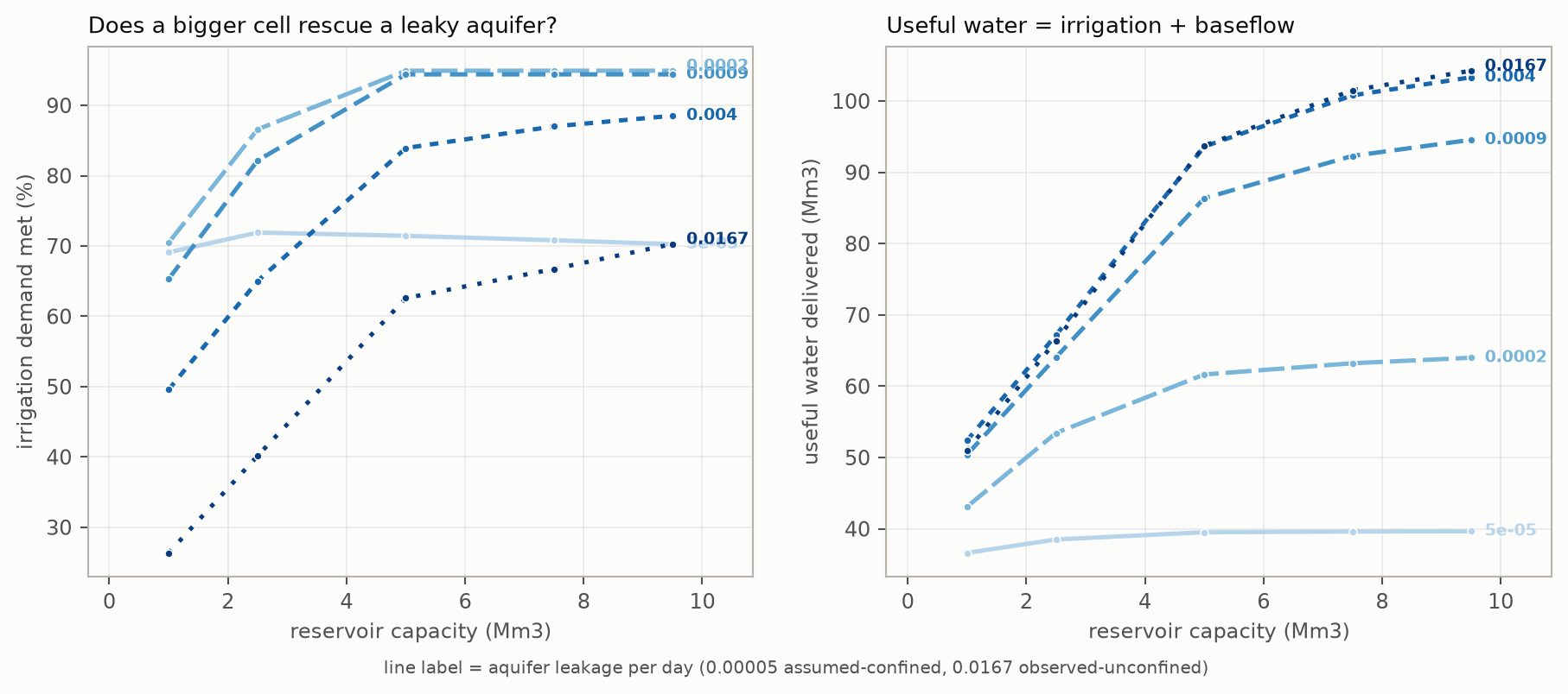
Figure 4. Irrigation reliability (left) and total useful water (right) against the size of the surface cell, with one line per leakage value. Does not show: construction feasibility, ground conditions, or any cost.
The lines cross, and that is the finding. For a leaky store, a bigger cell is transformative — reliability climbs from 26% to 70% as the cell grows from 1 to 9.5 Mm³. For a tight store it does almost nothing: the top line is flat, and even declines slightly, peaking at 2.5 Mm³.
The reason is that the two configurations are limited by different things. A leaky store is short of water, so more water helps. A tight store fills up and stays full — it is short of room, and a bigger surface cell cannot give it any.
So “how big should the reservoir be?” has no answer until you know how the aquifer behaves. If it is tight, 2.5 Mm³ is enough and anything larger is wasted. If it leaks at the observed rate, every cubic metre the terrain allows is worth having.
6.2 Evaporation is a property of the site
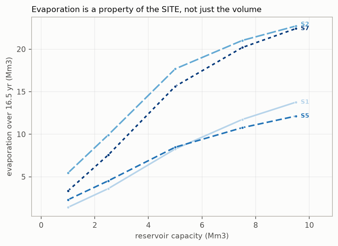
Figure 5. Evaporation over the record against cell capacity, one line per candidate site. Does not show: seepage into the ground, which is separate and unquantified.
The same volume of water evaporates at very different rates depending on where it is put. At 5 Mm³, the best-shaped site loses 8.3 Mm³ over the record; the flattest loses 17.7 Mm³ — more than double, for the same stored volume. A shallow cell spread across the moor has far more surface exposed to the sun.
This is a real cost of the flat-ground siting that Figure 2 already disfavoured on embankment grounds. The moor sites lose twice.
6.3 How much underground storage is needed
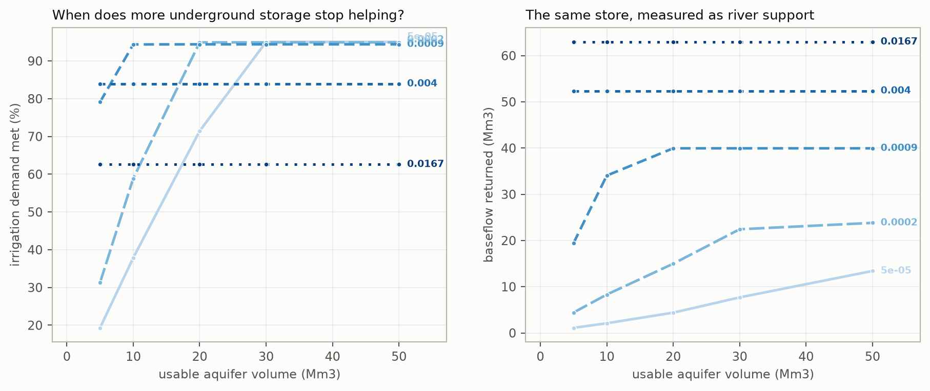
Figure 6. Reliability (left) and baseflow returned (right) against usable aquifer volume, one line per leakage value. Does not show: whether any such volume exists beneath the site — this is exactly the quantity nobody has measured.
This is the most important figure in the paper, and the lines invert.
- With only 5 Mm³ of usable storage, the tight aquifer is the worst option, meeting 19% of demand — while a moderately leaky one meets 79%.
- With 30 Mm³, the tight aquifer is the best, at 95%.
A tight store that is too small fills up in the first wet winter and refuses everything after that; the water sits in the reservoir and evaporates. A leaky store empties itself and is always ready to take more — which is useless for summer supply but keeps the scheme moving.
So the sentence “a confined aquifer is better” is only true above about 20 Mm³ of usable volume. Below that it is false, and badly so. Which of those worlds we are in is not known.
The right-hand panel shows the same runs measured at the river: baseflow rises with leakage, monotonically. The two products trade against each other.
6.4 Recovery capacity
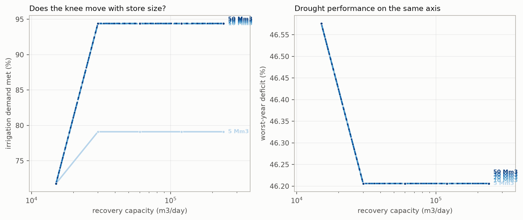
Figure 7. Reliability and worst-year deficit against the capacity to pump water back out, one line per aquifer volume. Does not show: whether a real wellfield could achieve these rates — the aquifer properties that would determine it are the unmeasured ones.
The knee does not move. At every store size, reliability rises sharply to 30,000 m³/day and then stops dead — 60,000, 120,000 and 240,000 give exactly the same answer. What does move is the level the knee reaches: 79% with a 5 Mm³ store, 94% with 10 Mm³ or more.
This is a clean null result on a design lever. Beyond 30,000 m³/day, recovery plant is wasted money in every scenario tested. The constraint past that point is whether the water is in the ground on the day it is wanted, which no amount of pumping capacity fixes.
6.5 Injection capacity
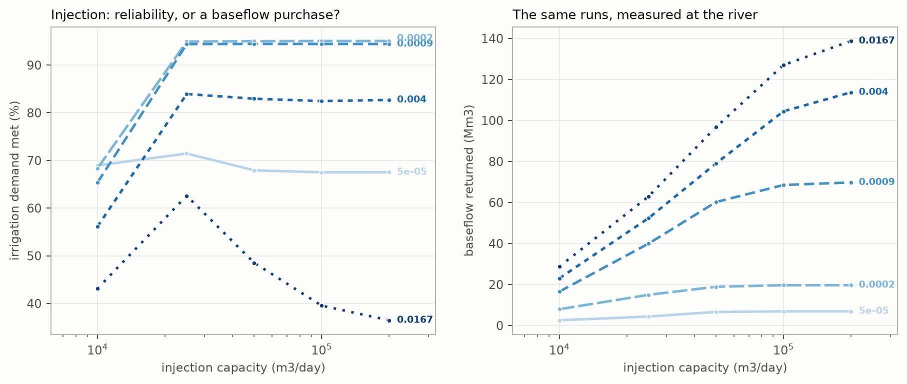
Figure 8. Reliability (left) and baseflow (right) against the capacity to inject water underground, one line per leakage value. Does not show: well clogging, which is the classic failure mode of injection schemes and is not modelled anywhere.
More injection capacity makes a leaky store worse. The bottom line peaks at 25,000 m³/day and then falls away — from 63% down to 37% as capacity is raised eightfold. Water is pushed underground faster, and a leaky store simply leaks it away faster, having drained the reservoir that could have supplied it later.
For a moderately tight store the picture reverses: reliability climbs to 95% and then saturates.
Meanwhile baseflow rises steeply and monotonically in every scenario, up to 139 Mm³. Injection capacity is mostly a purchase of river support, not of irrigation reliability — and in the leaky case, buying more of the first actively costs you the second.
6.6 Diversion pump capacity
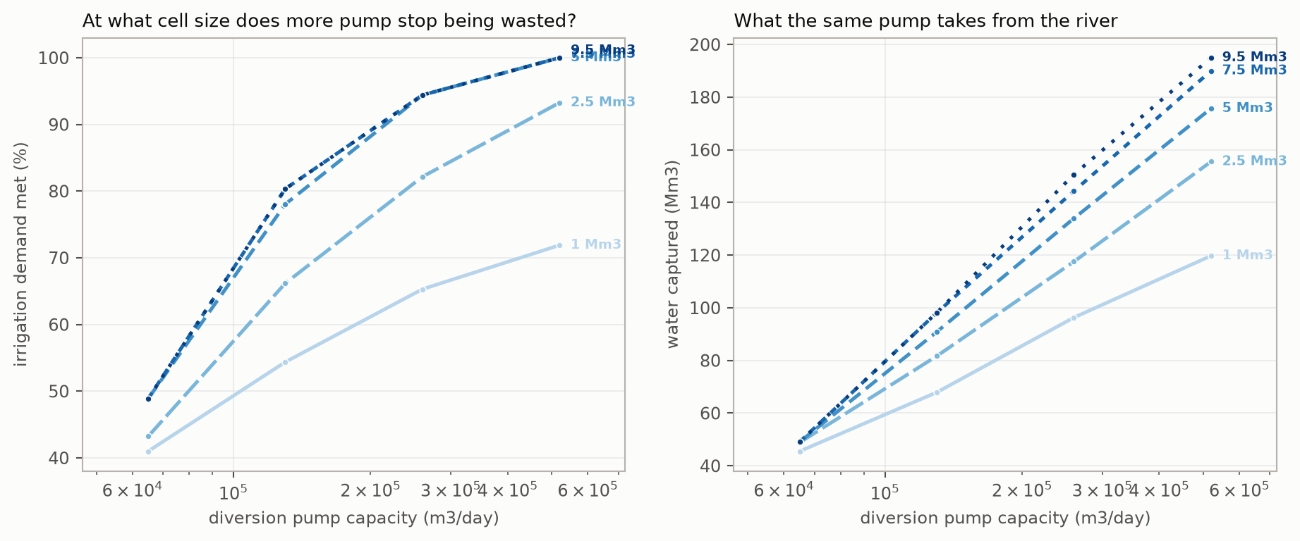
Figure 9. Reliability and total water captured against the diversion pump, one line per reservoir capacity. Does not show: the licence implications of taking more water, or intake works.
A bigger pump only pays if there is somewhere to put the water. With a 1 Mm³ cell, quadrupling the pump raises reliability from 41% to 72%. With a 5 Mm³ cell the same change takes it from 49% to 100%. The lines fan apart: pump and cell have to be sized together.
At the largest pump tested the scheme meets demand in full — but it takes 176 Mm³ from the river to do it, against 134 Mm³ at the baseline. The licence rule is unchanged; the scheme is simply taking more on every day that qualifies. Whether that would be acceptable is a regulatory question this study cannot answer.
7. The drought-timing question
The only severe drought in the record falls in 2011 — near the start, when the stores are still filling from empty. Measured deficits there are part drought and part start-up, and the two cannot be separated from a single record.
So the same sixteen years were run twice: once as recorded, and once with the first three water years moved to the end, so the identical drought is met by a scheme that has been cycling for a decade.
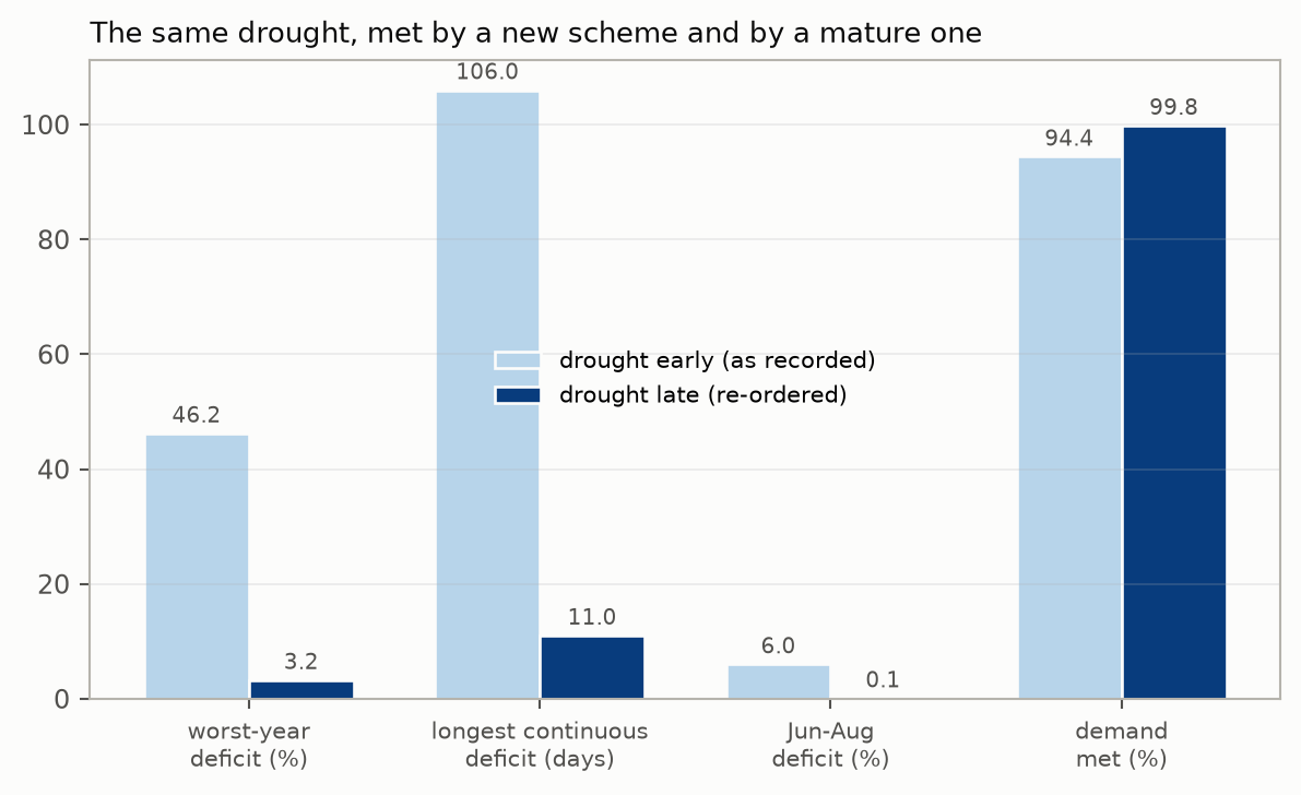
Figure 10. The same drought met by a new scheme and by a mature one. Does not show: any change in the weather — the two runs contain identical years in a different order.
| drought early (as recorded) | drought late (re-ordered) | |
|---|---|---|
| Worst-year deficit | 46.2% | 3.2% |
| Longest continuous shortfall | 106 days | 11 days |
| June–August deficit | 6.0% | 0.1% |
| Demand met | 94.4% | 99.8% |
This is a range, not a correction. Both numbers are true answers to different questions. A scheme commissioned in 2009 genuinely would have met the 2011 drought with empty stores, and would genuinely have failed that badly. A scheme that had been running for a decade would have sailed through.
The honest reading: almost all of the baseline’s apparent drought weakness is a start-up effect. Confirming this, the driest three consecutive years in the record (2015–2017), which the scheme meets with full stores, produce no deficit at all in the baseline.
What re-ordering breaks. Each year keeps its own weather, but the sequence between years is destroyed — a dry year no longer follows the wet one that actually preceded it. Multi-year drought behaviour, which is what most threatens a store like this, cannot be tested from a record containing only one severe event. Sixteen years is not enough to characterise drought risk, and no rearrangement of it will be.
8. The best realistic option
On the evidence above, the configuration that survives the most scenarios:
| Element | Value | Reason |
|---|---|---|
| Reservoir | 5–7.5 Mm³ at the best-shaped site | Above 5 Mm³ gains are small unless the aquifer is leaky; the terrain caps it at 9.9 |
| Recovery | 30,000 m³/day | The knee, in every scenario |
| Injection | 25,000 m³/day | More is harmful if the store is leaky, neutral if not |
| Diversion pump | 260,000 m³/day | Larger works, but takes materially more river water |
| Aquifer | seek ≥ 20 Mm³ usable | Below this, a tight store is the worst option, not the best |
Physically, at 5 Mm³:
| Quantity | Baseline (8 km store) | Distant store (42 km) |
|---|---|---|
| Pipeline | 11.5 km | 45.5 km |
| Total pumping head | 29.8 m | 78.6 m |
| Pipe diameter | 1.60 m | 1.60 m |
| Installed pumping power | 1,258 kW | 3,316 kW |
| Annual pumping energy | 0.78 GWh | 1.59 GWh |
| Embankment fill | 78,000 m³ | 78,000 m³ |
| Injection wells | 25 | 25 |
| Recovery wells | 15 | 15 |
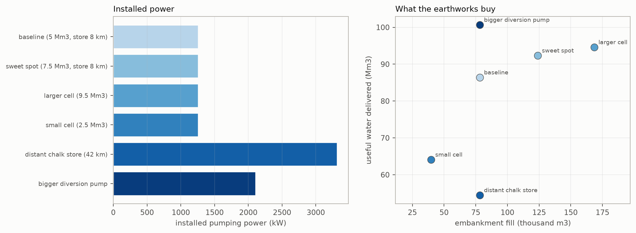
Figure 12. Installed power by configuration, and useful water delivered against embankment fill. Does not show: any cost — unit rates for earthworks, pipe and plant are not open data, and inventing them would put a spurious number at the front of this paper.
Well counts assume each injection well accepts 1,000 m³/day and each recovery well yields 2,000 m³/day. Both are assumptions with no measurement behind them, and they are precisely the numbers a pumping test would establish. If real acceptance were half the assumption, the well count doubles.
Going to the distant store doubles the energy and quadruples the pipeline for very similar irrigation delivery — 46.7 Mm³ against 46.4 — but collapses baseflow from 39.9 to 7.7 Mm³. That is not a small difference in a co-product; it is most of one product gone.
How the picture moves, and what to look for
If the aquifer is tight and large (≥ 30 Mm³ usable): reliability 95%, worst year comfortable, baseflow small (4–8 Mm³). A summer-supply scheme.
If the aquifer is tight but small (5 Mm³): reliability 19%. The scheme does not work in this form, and no amount of reservoir or plant fixes it.
If the aquifer leaks at the observed rate: reliability 63%, baseflow 63 Mm³. A river-support scheme that also irrigates, and one that wants the largest cell the terrain allows.
The inverse statement, which is the useful one. If 20–30 Mm³ of usable, reasonably tight storage could be found anywhere within reach — under this site or another — the scheme delivers 94–95% of irrigation demand with a 5 Mm³ surface cell and modest plant. That is a specific thing to go looking for, and it is a more productive question than asking whether this particular site is difficult.
9. Adding a second aquifer
Everything so far uses one store. A second store of different character can be added, splitting the recharge between them.
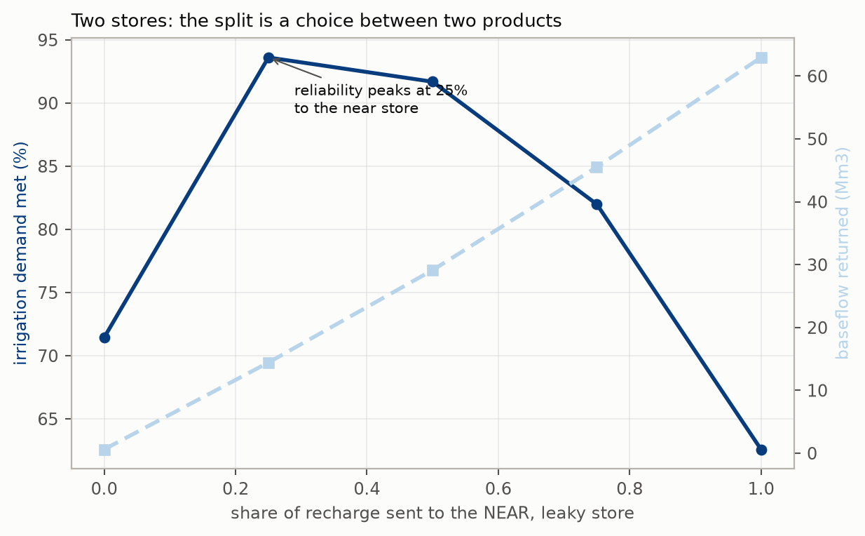
Figure 11. Irrigation reliability and baseflow against the share of recharge sent to the near, leaky store. Does not show: the cost of the second pipeline and wellfield, which is substantial and unpriced.
| Share to the near, leaky store | Demand met | Baseflow |
|---|---|---|
| 0% (all to the tight store) | 71.4% | 0.6 Mm³ |
| 25% | 93.6% | 14.4 Mm³ |
| 50% | 91.7% | 29.1 Mm³ |
| 75% | 82.0% | 45.5 Mm³ |
| 100% | 62.6% | 63.0 Mm³ |
Reliability does not fall steadily as water is diverted to the leaky store — it peaks at 25% and is worse at 0% than at 25%. Sending everything to the tight store is not the reliability optimum, because a store that fills and stops accepting water is worth less than two stores that keep cycling.
Baseflow, by contrast, rises steadily throughout. So the split is a genuine choice between two products, with one point (25%) that is better than the extremes for irrigation while still returning 14 Mm³ to the river.
This is a refinement, not the base case. It requires a second pipeline and a second wellfield, and it should only be considered once the single-store question — how the first aquifer actually behaves — has been answered.
10. What “useful” means, and what constrains it
The scheme makes two products that do not convert into each other: water delivered to crops in summer, and water returned to the river in dry weather. There is no defensible exchange rate between them, and this paper does not invent one. Any monetary value placed on river support would be made up, and would then carry the whole answer.
The trade-off is real and it runs through every result. A tight store banks water for irrigation and returns almost nothing to the river. A leaky store supports the river and struggles to hold water to August. Which is “better” depends entirely on what the scheme is for — and that is a decision for people, not for a model.
What actually constrains this scheme
In order:
- Not knowing how the aquifer behaves. Reliability spans 19% to 95% across the range of what is not known.
- The size of the usable underground store, which inverts the answer to question 1.
- The terrain. The best surveyed site holds 9.9 Mm³ and no more.
- The recovery plant — but only up to 30,000 m³/day, after which it is not a constraint at all.
Notice what is not on that list: the river. The catchment has far more divertible water than the scheme can use, and this has been true in every test. Water availability is not the binding constraint on this scheme, and never was.
The inverse statements
Rather than only reporting that something is hard, these say what would have to be true for it to be easy:
- If 20–30 Mm³ of usable, low-leakage storage exists within about 10 km, the scheme works well — 94–95% reliability on a 5 Mm³ cell.
- If a site with the shape of the unsurveyed candidate C1 is real, it stores 30% more water per cubic metre of bank than anything surveyed, with a quarter of the lift and less than half the conveyance. Roughly 40 LiDAR tiles would settle it.
- If injection acceptance is half what has been assumed, the wellfield doubles from 25 to 50 wells, and injection capacity would need rethinking — but Figure 8 shows more injection is not what the scheme needs anyway.
11. Conclusions and recommendations
-
The scheme is physically plausible and the river can supply it. The baseline delivers 46 Mm³ of irrigation and 40 Mm³ of river support over sixteen and a half years, meeting 94% of demand.
-
The reported reliability hides the shape of the failures. The same run misses 46% of one year’s demand and runs a 106-day continuous shortfall. Report deficits, not averages.
-
Most of that apparent weakness is a start-up effect. Met by a scheme that had been running a decade, the same drought produces a 3.2% worst year and an 11-day shortfall. Both numbers are real; they answer different questions.
-
The dominant uncertainty is not a design choice. How the aquifer behaves, and how much usable volume it has, together span 19% to 95% reliability. Every design lever in this paper is small beside that.
-
The ranking of options inverts across that uncertainty. A tight aquifer is the best choice above about 20 Mm³ of usable volume and the worst below it. A bigger reservoir is transformative for a leaky store and wasted on a tight one. No configuration can be recommended without the measurement.
-
Two clean null results. Recovery capacity beyond 30,000 m³/day changes nothing in any scenario tested. Extra injection capacity buys river support, not reliability — and in a leaky store it actively reduces reliability.
-
The terrain has been more informative than expected. Flat ground is bad for storage twice over: five times the embankment and double the evaporation. The best sites are in hollows at the moor’s edge, not on the moor.
Recommendations
First, measure the aquifer. A test borehole and a pumping test on the local sandstone would establish leakage, usable volume, and well acceptance — the three quantities that between them determine whether this works. Nothing else in this paper is worth optimising until they are known, and the range of outcomes they span is larger than the difference between any two configurations considered here.
Second, complete the terrain survey where it is cheap to do so. The best site found anywhere sits in a gap in the existing LiDAR, inside the area already flown. Roughly forty tiles would confirm or dismiss it.
Third, decide what the scheme is for. Irrigation supply and river support pull in opposite directions and no analysis can choose between them. That decision changes which aquifer to target and how big to build.
Fourth, do not present this as flood management. The peak reduction is 1–2% and the ceiling is arithmetic.
APPENDIX A: Terms and abbreviations
Written for readers coming from any of hydrology, hydrogeology, mapping or water regulation — no one reader is expected to know all four.
AOD — Above Ordnance Datum. Height above mean sea level as used on British maps. “14 m AOD” means 14 m above sea level.
Aquifer — Rock that holds and transmits usable amounts of water.
ASR — Aquifer Storage and Recovery. Putting water into an aquifer specifically to take the same water out later. The narrower case of MAR.
Baseflow — The portion of river flow sustained by water draining out of the ground, rather than by recent rain. It keeps rivers running in dry weather.
BGS — British Geological Survey. The UK’s national geological organisation.
Confined aquifer — An aquifer sealed above by a layer that water cannot easily pass through. Water is held under pressure and cannot escape upward, so a confined store retains water far better.
Deficit distribution — Reporting shortfall by how it is spread — worst single year, how many years exceed a threshold, how long a continuous shortfall lasts — rather than as one overall percentage. A scheme “94% reliable” can still fail badly in the year that matters.
DEM / DTM — Digital Elevation Model / Digital Terrain Model. A grid of ground heights. A 50 m DEM has one height every 50 m.
EA — Environment Agency. The regulator for water in England, and the source of the river-flow data here.
Embankment efficiency — Cubic metres of water stored per cubic metre of earth bank needed to retain it. Higher is better. It rises with size and falls with depth, so wide and shallow beats narrow and deep — but wide and shallow evaporates more.
Evapotranspiration / PET — Water lost to the air from open water, soil and plants. Potential evapotranspiration is the loss if water were freely available.
Exceedance — How often a flow is equalled or exceeded. The “12.5% exceedance flow” is the flow the river beats one day in eight. Using exceedances rather than fixed numbers keeps a rule equally strict on different rivers.
Fracture flow vs intergranular flow — Two ways water moves through rock. Intergranular: through the pore spaces between grains, like a sponge — predictable, and what most of this paper’s storage assumes. Fracture: through cracks — fast, hard to predict, and water can travel a long way quickly.
Hands-off flow — The river flow below which abstraction must stop entirely. A licence floor protecting the river.
LiDAR — Laser survey from aircraft, giving very detailed ground heights (1 m here). Accurate but expensive, so coverage is patchy.
MAR — Managed Aquifer Recharge. Deliberately putting water into an aquifer for later use or to support the environment.
Mm³ — Million cubic metres. One Mm³ is 1,000,000,000 litres, roughly 400 Olympic swimming pools.
NRFA — National River Flow Archive. The UK’s curated archive of river-flow records and gauging-station catchment data.
NSE — Nash–Sutcliffe Efficiency. A score for how well a model reproduces observations. 1.0 is perfect; 0 means no better than using the average.
Q12.5, Q19 — Shorthand for exceedance flows: Q12.5 is the flow exceeded 12.5% of the time. Higher percentages mean lower flows.
Ramsar site — A wetland of international importance, protected under the Ramsar Convention.
Recession — The way a water level falls once input stops. Its half-life is how long the level takes to fall halfway back — 41 days in the local unconfined boreholes, which is fast.
SAC / SPA — Special Area of Conservation / Special Protection Area. Habitat and bird designations carrying the strongest legal protection in England.
Specific yield — The fraction of a rock’s volume that will actually drain out under gravity. It converts rock volume into usable water volume, and is one of the unmeasured quantities.
Spin-up — The early part of a simulation while stores fill from their starting state. Results during spin-up reflect the starting condition as much as the system.
SPZ — Source Protection Zone. Ground around a public water-supply borehole where activities are restricted. Zone 1 is the innermost and most restrictive.
SSSI — Site of Special Scientific Interest. The main national wildlife and geology designation in Britain.
Storativity / storage coefficient — How much water an aquifer releases per unit drop in water level. With transmissivity, it determines how a store behaves. Not published for this aquifer.
Transmissivity — How readily an aquifer transmits water horizontally. Determines how fast water can be injected or recovered. Not published for this aquifer.
Unconfined aquifer — An aquifer open to the surface above, its water table free to rise and fall. Easier to recharge, much leakier.
Water year — A twelve-month period starting 1 October, used so that a winter and the following summer fall in the same year rather than being split across two.
WFD — Water Framework Directive. The regulatory framework classifying water bodies and setting objectives for them.
APPENDIX B: Additional figures
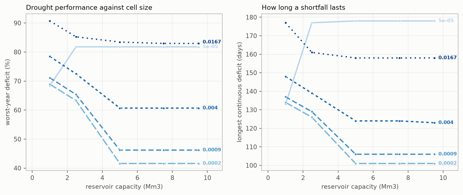
Figure 13. Worst-year deficit and longest continuous shortfall against reservoir capacity, one line per leakage value — the drought counterpart to Figure 4. Does not show: multi-year drought behaviour, which this record cannot test.
APPENDIX C: Full parameter table
Baseline values, and the range each takes across the sensitivity runs. 141 runs in total; worst mass-balance error 0.000002 m³.
| Parameter | Baseline | Range tested | Status |
|---|---|---|---|
| Simulation period | 2010-01-01 to 2026-06-30 | fixed | measured |
| Inflow gauges | 8 | fixed | measured |
| Mean river flow | 14.55 m³/s | — | measured |
| Diversion trigger | 30.58 m³/s (Q12.5) | fixed | derived |
| Hands-off flow | 21.21 m³/s (Q19) | fixed | derived |
| Low-flow support threshold | 3.84 m³/s (Q73.1) | fixed | derived |
| Diversion pump | 260,000 m³/day | 65,000 – 520,000 | assumed |
| Reservoir site | best surveyed | 4 sites | terrain |
| Reservoir capacity | 5 Mm³ | 1 – 9.5 Mm³ | terrain-capped |
| Reservoir area | from stage curve | per site | terrain |
| Treatment efficiency | 0.98 | fixed | assumed |
| Injection capacity | 25,000 m³/day | 10,000 – 200,000 | assumed |
| Aquifer usable volume | 20 Mm³ | 5 – 50 Mm³ | unmeasured |
| Aquifer leakage | 0.0009 /day | 0.00005 – 0.0167 | scenario bounds |
| Leakage credited to river | 0.8 | fixed | assumed |
| Recovery capacity | 30,000 m³/day | 15,000 – 240,000 | measured knee |
| Recovery efficiency | 0.6 | fixed | assumed |
| Conveyance distance | 8 km | 8 / 42 km | measured |
| Irrigation demand | 3 Mm³/year | fixed | specified |
| Autumn drawdown | 2.5 Mm³, Oct–Nov | fixed | assumed |
| Pipe design velocity | 1.5 m/s | fixed | assumed |
| Pump efficiency | 0.70 | fixed | assumed |
| Injection well acceptance | 1,000 m³/day | fixed | assumed |
| Recovery well yield | 2,000 m³/day | fixed | assumed |
Every row marked assumed or unmeasured is a candidate for the measurement programme recommended in Section 11. The rows that matter most are aquifer leakage and usable volume.
All analysis from openly published data. Contains Environment Agency and Natural England information © and/or database right, Open Government Licence v3; British Geological Survey materials © UKRI; Ordnance Survey data © Crown copyright and database right.