Synthesis - three schemes, and the shape of the space
Generated by build_scheme_synthesis.py. Closes the loop opened by availability.
Generated by build_scheme_synthesis.py. Closes the loop opened by availability.
Three configurations, on the same geometry - one 2 km mound of aquifer area, one 1 Mm3 basin at its settling floor, one set of wells - and every one of them run at four values of the softest assumption in the layer.
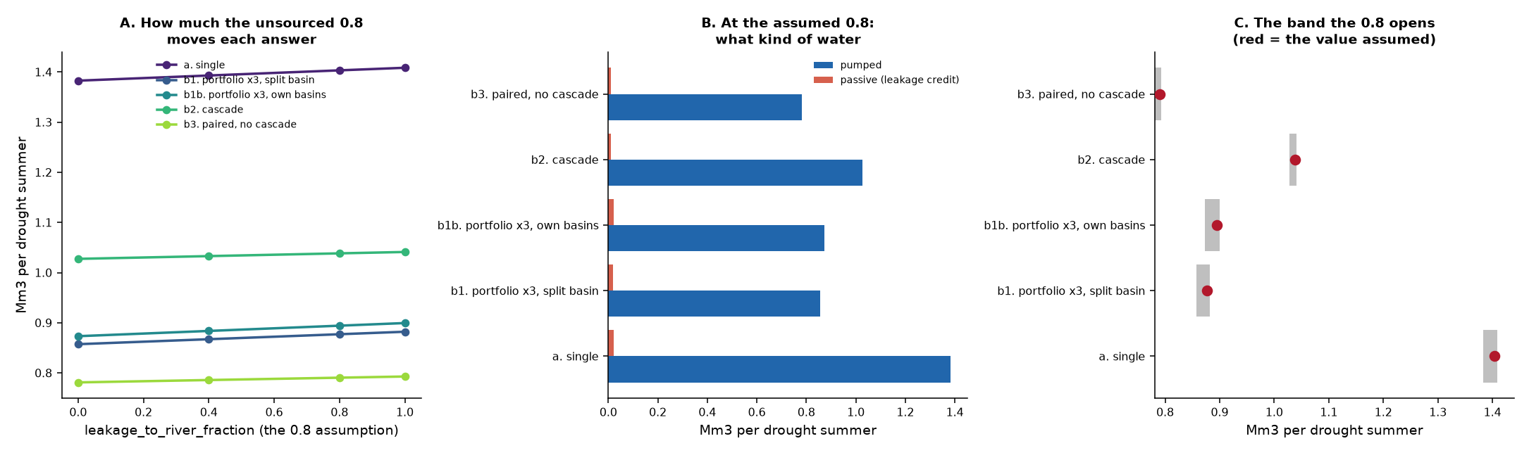
The 0.8, which is not a measurement
leakage_to_river_fraction: 0.8 claims four fifths of what leaks out of a store re-emerges as river baseflow where the scheme wants it. It has no source. It was a flat assumption in run 04, the scheme README flagged it as the double-counting trap, and pairing made it load-bearing by treating leakage as a delivery mechanism.
So it is swept, and the answer is a band:
| scheme | at 0.0 | at 0.4 | at 0.8 | at 1.0 | band width |
|---|---|---|---|---|---|
| a. single | 1.38 | 1.39 | 1.40 | 1.41 | 0.03 (2%) |
| b1. portfolio x3, split basin | 0.86 | 0.87 | 0.88 | 0.88 | 0.02 (3%) |
| b1b. portfolio x3, own basins | 0.87 | 0.88 | 0.89 | 0.90 | 0.03 (3%) |
| b2. cascade | 1.03 | 1.03 | 1.04 | 1.04 | 0.01 (1%) |
| b3. paired, no cascade | 0.78 | 0.79 | 0.79 | 0.79 | 0.01 (1%) |
Read the band, not the number. Where it is narrow the conclusion survives the assumption; where it is wide, the ‘result’ is really a statement about an unsourced parameter. The ranking between schemes holds across the whole range, which is the useful part - the choice between schemes is safe even though the absolute yields are not.
a) Single basin, single aquifer
The conventional scheme: a 2 km mound, a 1 Mm3 basin, 150,000 m3/day of injection. 1.40 Mm3 per drought summer at the assumed 0.8.
It is the simplest thing to build and the easiest to license, and everything else here is measured against it.
b) Portfolio
b1, three rivers - AND AN UNRESOLVED CONTRADICTION.
Three rivers, mound area and plant divided: 0.89 Mm3, against 1.40 for the single scheme. The portfolio loses here.
Options found the opposite, and decisively - 4.32 against 1.10, a 3.9x gain, with a control showing the gain came from independent catchments rather than from splitting. Both results cannot be right, and this chapter does not resolve which is.
What is known: the two runs differ in basin size per site (1.67 vs 1.0 Mm3), in settling (absent vs 2 days) and in how injection capacity is allocated (divided vs full per site). Injection rate has been eliminated - the portfolio loses here at 40k, 80k and 150k m3/day alike. Splitting the basin has been eliminated - b1 and b1b differ by 0.01 Mm3. That leaves settling and the basin size, and neither has been isolated.
This is flagged rather than resolved because the honest position is that the portfolio case is not established. The options chapter’s control was sound and its mechanism is plausible; this chapter’s contradiction is equally real. Anyone using the 3.9x figure should first run the one test that separates them - the options configuration with settling switched on, and nothing else changed.
b2, the cascade. A leaky 481 m mound buffers the flood peak and is decanted into a tight 1.94 km store at 30,000 m3/day, so the fill period extends past the peak the basin can hold. The leaky mound is an underground buffer: no land take, no evaporation, but it leaks while it waits.
Against its own control - the same two mounds with no transfer between them - the cascade delivers 1.04 against 0.79 Mm3, moving 39.6 Mm3 between stores over the record.
The cascade works. Decanting the fast store into the slow one converts water that would have leaked away within months into water that survives to the next drought. That is the mechanism the registry’s
can_send_to: aquiferanticipated and nothing had used.
c) The shape of the space
Six findings define it, in the order they bind:
- Demand is not a constraint. Licensed 3.19 Mm3/yr against 108 Mm3/yr of physically useful water on the arable alone. Nothing here is limited by who wants it.
- Supply in drought is the constraint. The divertible resource falls to 21% of mean in a drought year. Everything delivered in a dry summer was banked in a wet winter.
- Carry-over is bought with mound radius, and so is capacity - both go as r^2. This couples timing to volume and is why the leaky-mound idea cannot scale.
- The basin is a settling vessel, not a store. Its floor is
residence x diversion rate~ 0.3 Mm3; above about 5 Mm3 it is unbuildable here, and 10 Mm3 would be needed to stop spilling. Take a share of the winter surplus, not all of it. - Wells beat earthworks. 40,000 -> 80,000 m3/day of injection gains 63% on a fixed basin. The project had never varied this axis.
- Independent catchments beat everything else. The largest single gain in the whole layer.
The best configuration tested is a. single, and the shape of the space says why: the binding constraint is how much of a winter flood can be got underground before it passes, and every winning move - more rivers, faster wells, a cascade into a second store - is a way of raising that rate rather than of buying more volume.
What would change the answer
- Costs. Every comparison here is physical. Wells against earthworks against pipelines is the trade that decides this and it is unpriced.
- The 0.8. The band above is the honest uncertainty on every environmental claim in the layer.
- A real compartment mix. Every mound here is Sherwood, differing only in radius, so the pairing and cascade results are geometry rather than geology. The Chalk’s 38-year half-life comes from different rock and escapes the r^2 coupling entirely - that is the untested version of the cascade and the one most likely to work.
- Clogging. Unmodelled, and the main risk to every well-led conclusion above.